The Receiver Operating Characteristic (ROC) curve of a binary classification model describes all operating points obtainable by shifting the prediction threshold. Each operating point is characterized by a true positive rate (TPR, i.e. the accuracy on positive examples) and a true negative rate (TNR, i.e. accuracy on negative examples).
For example, the following are ROC curves for a small ResNet trained and evaluated on the cat/dog subset of CIFAR-10. The traditional presentation is with TPR on the y-axis and false positive rate (1 - TNR) on the x-axis, but in this post I’ll prefer TNR vs TPR.
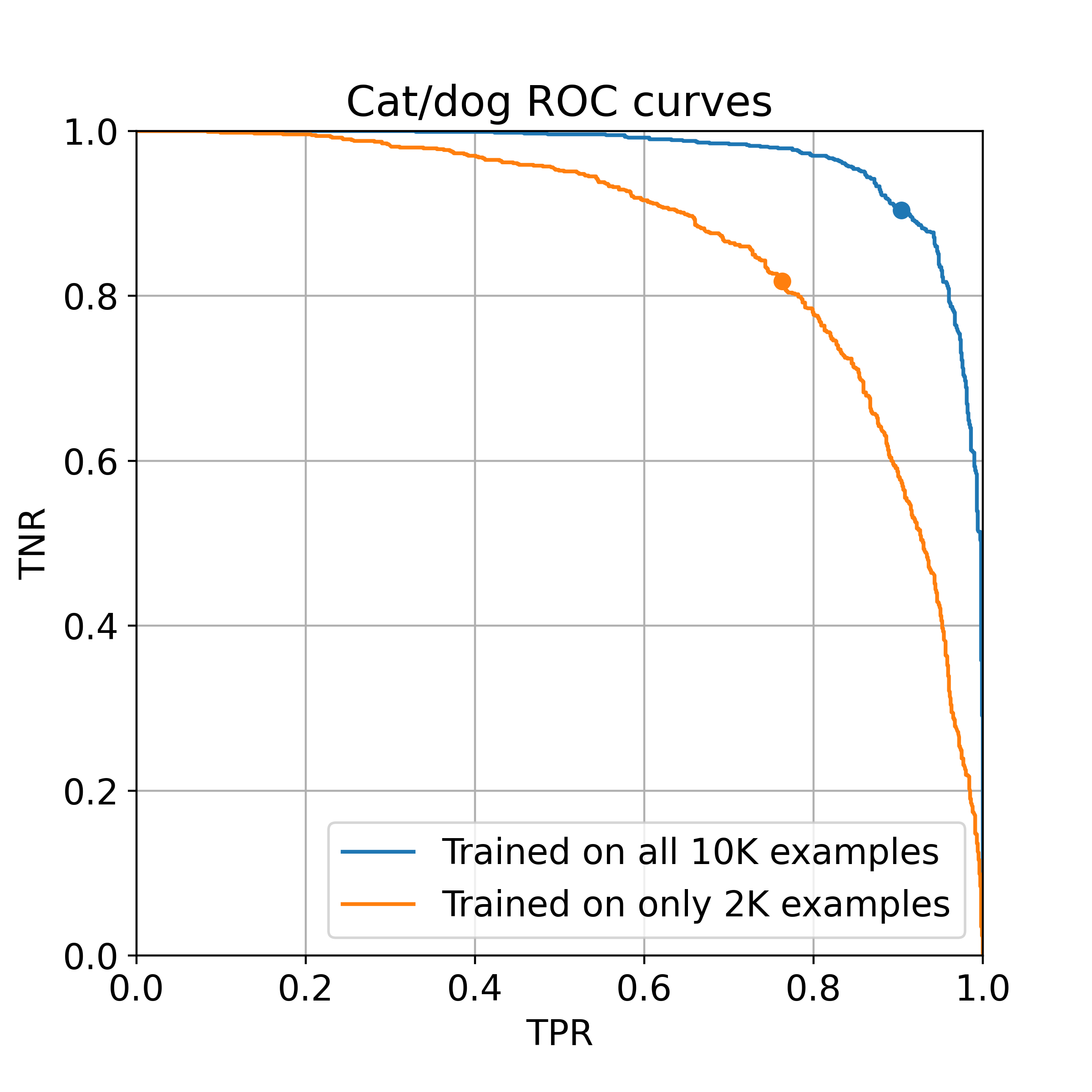
The dots indicate the operating point of the default threshold (i.e., predict cat when the softmax layer gives >50% probability to cat). The test-set is balanced, so that accuracy is simply given by $0.5 \cdot TPR + 0.5\cdot TNR$. Training on 2,000 examples gives a model with an accuracy of ~80%, and training on all 10,000 gives ~90%.
What’s more interesting to observe is that we can also operate the latter model at 50% TPR with nearly 100% TNR. This means that if we are fine with missing half of the positives (cats), then we can avoid almost all false-positives (dogs mispredicted as cat). This operating point corresponds to predicting “cat” only when the logit output of this model exceeds a threshold of 9.9.
In applied AI projects, this option to change the TPR/TNR tradeoff is crucial. For example, in many cases it’s necessary to have a TPR of nearly 100% so that no positive cases are missed, but false-positives are fine, since they will be passed through a more expensive and accurate second stage anyway. The reverse is equally common. In my work, it’s actually rare to operate a classifier at its default threshold.
Regularities
The science of deep learning proceeds by researchers identifying empirical regularities in the behavior of neural networks as a function of their size or training data. The most well-known examples are double descent and scaling laws.
I would like to present two regularities in the behavior of neural network ROC curves as a function of the training data. I feel it worthwhile to document these, although they may be intuitive or obvious in retrospect.
Each regularity will be demonstrated using a large-scale binary classification dataset, where we have 200K examples for validation, producing smooth curves. The training data contains 2M examples; our experiments will be done using smaller subsets. This is a proprietary text classification dataset on which we finetune BERT-type models; each experiment can however be easily replicated on academic or other datasets.
Shifting class balance induces crossed ROC curves
We’ll consider four different samples from a large pool of labeled examples.
- 50K positives + 50K negatives (100K total)
- 90K positives + 10K negatives (100K total)
- 10K positives + 90K negatives (100K total)
- 10K positives + 10K negatives (20K total, as a control)
We also consider three possible goals.
- Maximize overall (balanced) accuracy.
- Maximize TPR at 99.9% TNR. (i.e., max accuracy on positives, given that we can't misclassify more than 0.1% of negatives)
- Maximize TNR at 99.9% TPR. (i.e., max accuracy on negatives, given 99.9% accuracy on positives)
Our question is: Which class balance is optimal for each goal?
The answer can be decoded from the ROC curves for models trained on each dataset.
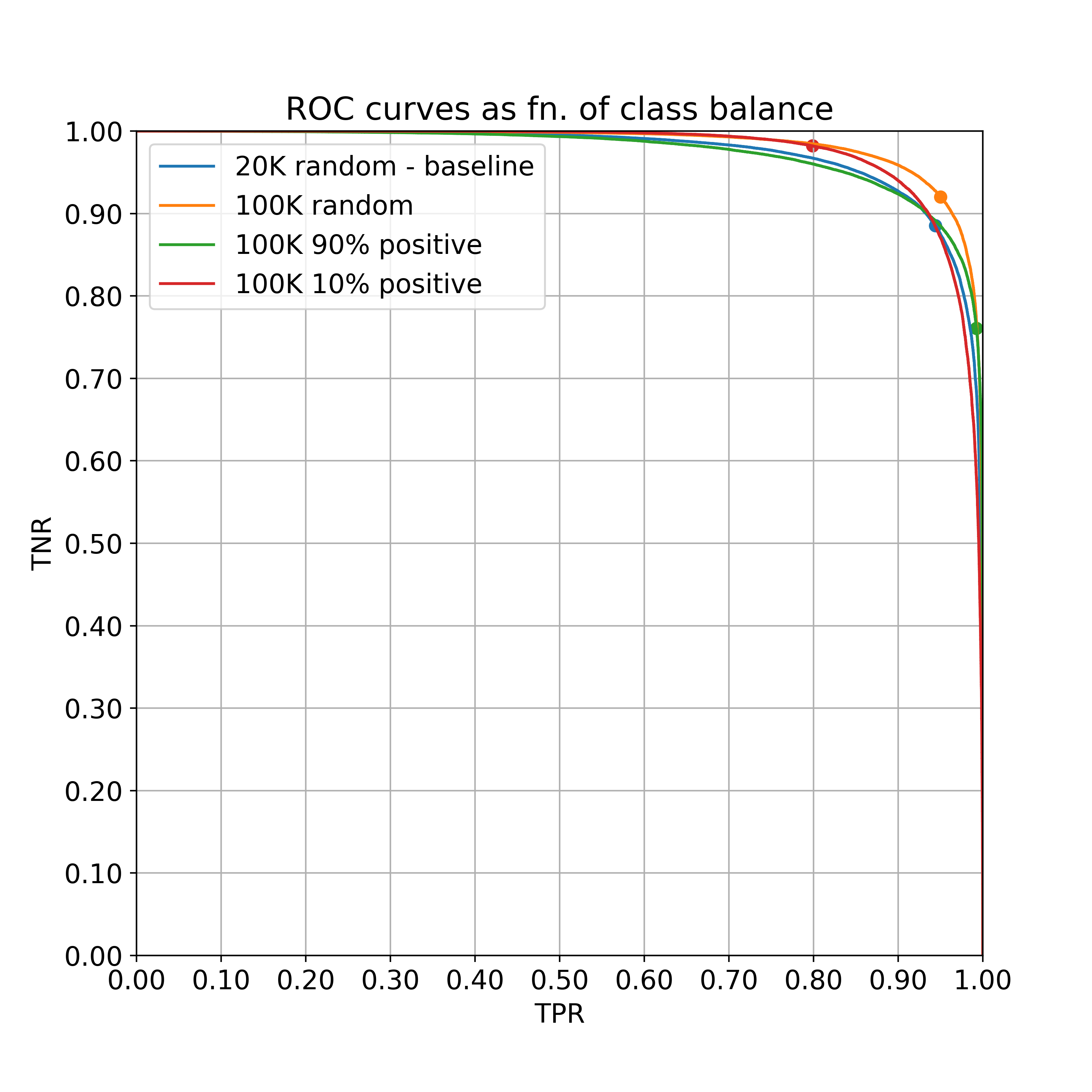
Let’s zoom into the top-right 25% to make this a bit easier to see.
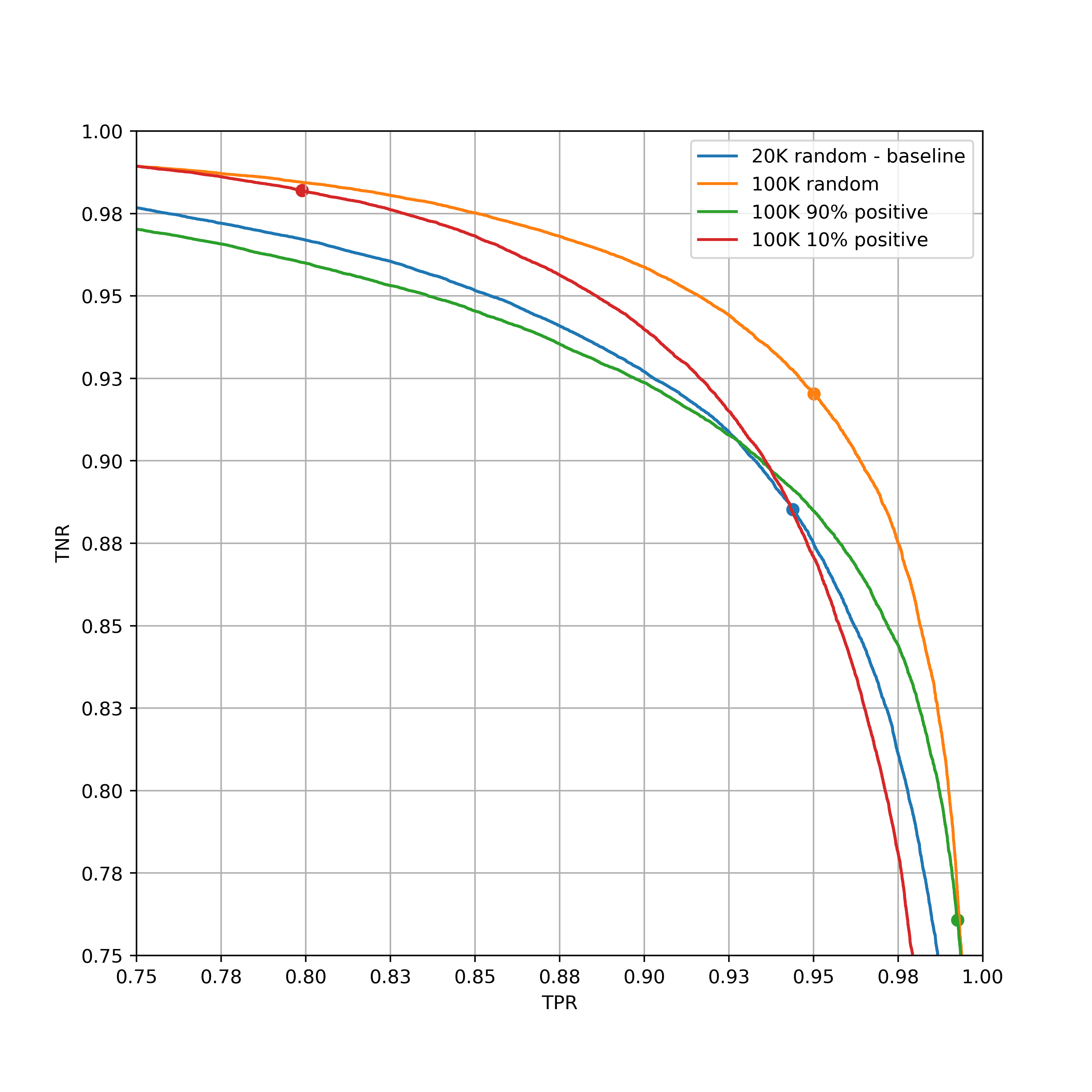
There is a clear takeaway: both the positive-heavy and negative-heavy samples are much worse than a balanced sample, for the purpose of overall accuracy. In fact, they yield (threshold-optimized) accuracies only around the baseline of 20K examples.
In addition, the positive-heavy set is clearly better than the negative-heavy set for the purpose of maximizing accuracy at a high TPR. And the negative-heavy set is clearly better when constraining to high TNR.
To see if these biased samples are ever better than the balanced sample, let’s switch the view to logistic-scale, which will let us more clearly see the ROC curves at TPRs and TNRs closer to 1.
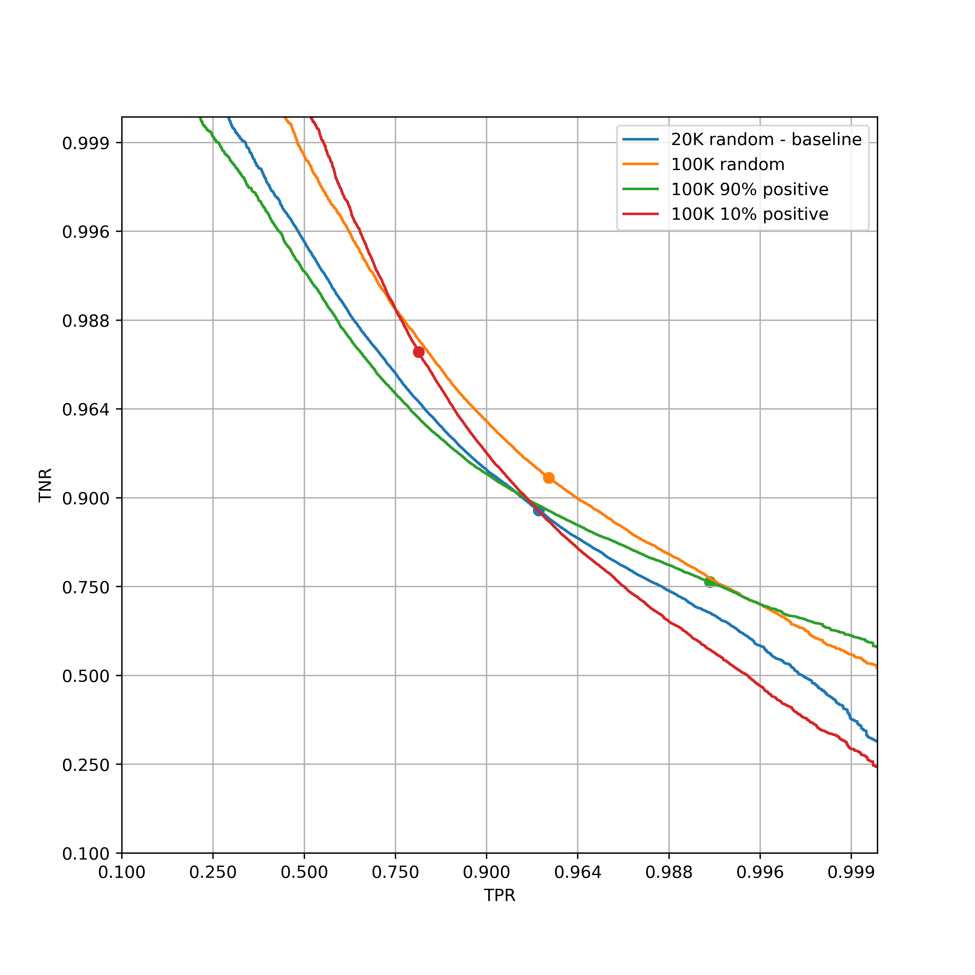
In this view, it becomes visible that the positive-heavy set is indeed better than a balanced sample when TPR is constrained to be at least 99.9%. Therefore, the answer to our question is:
- To max overall accuracy, the balanced distribution (1) is best.
- To max TPR at high TNR, sampling positive-heavy (3) is best.
- to max TNR at high TPR, sampling negative-heavy (2) is best.
This behavior is consistent across a wide range of architectures and datasets. The ROC curve is quite well-behaved as a function of the class balance and dataset size; it is possible to fit accurately-generalizing power laws to various aspects of the curve.
Label cleaning strategies target regions of the ROC curve
Next we can look at the effect of label noise on the ROC curve. We will have some intriguing observations. We will start with the following.
- Train on a baseline of 50K random samples, with clean labels.
- Flip 20% of the labels in this set (so 10K examples), and train a different model.
- Show the ROC curves for both.
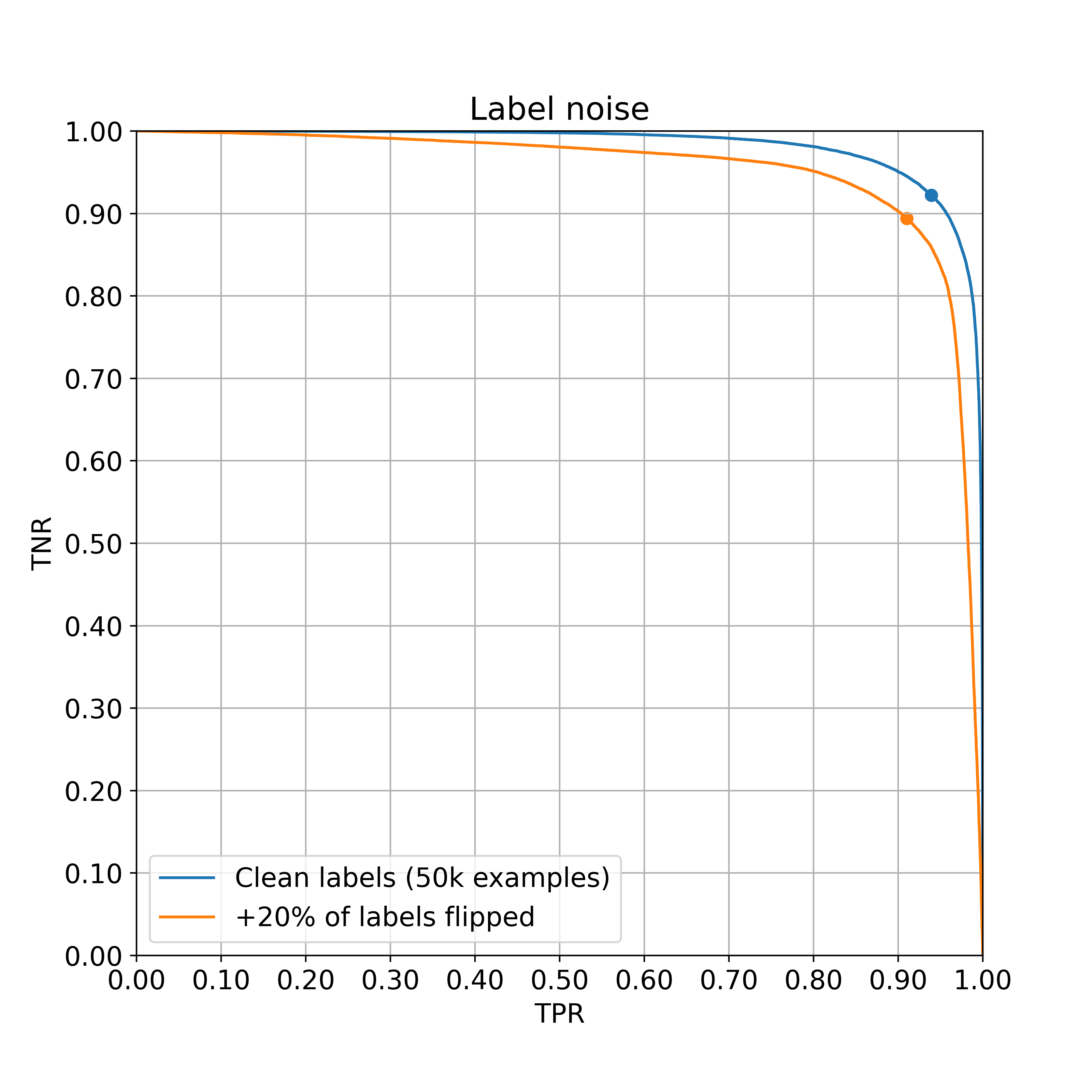
As expected, the label noise hurts performance, bringing balanced accuracy down from ~93% to ~90%. An even stronger effect, though, is that the performance constrained to high TPR or high TNR has declined significantly. This becomes even more clear when we visualize in logistic-scale.
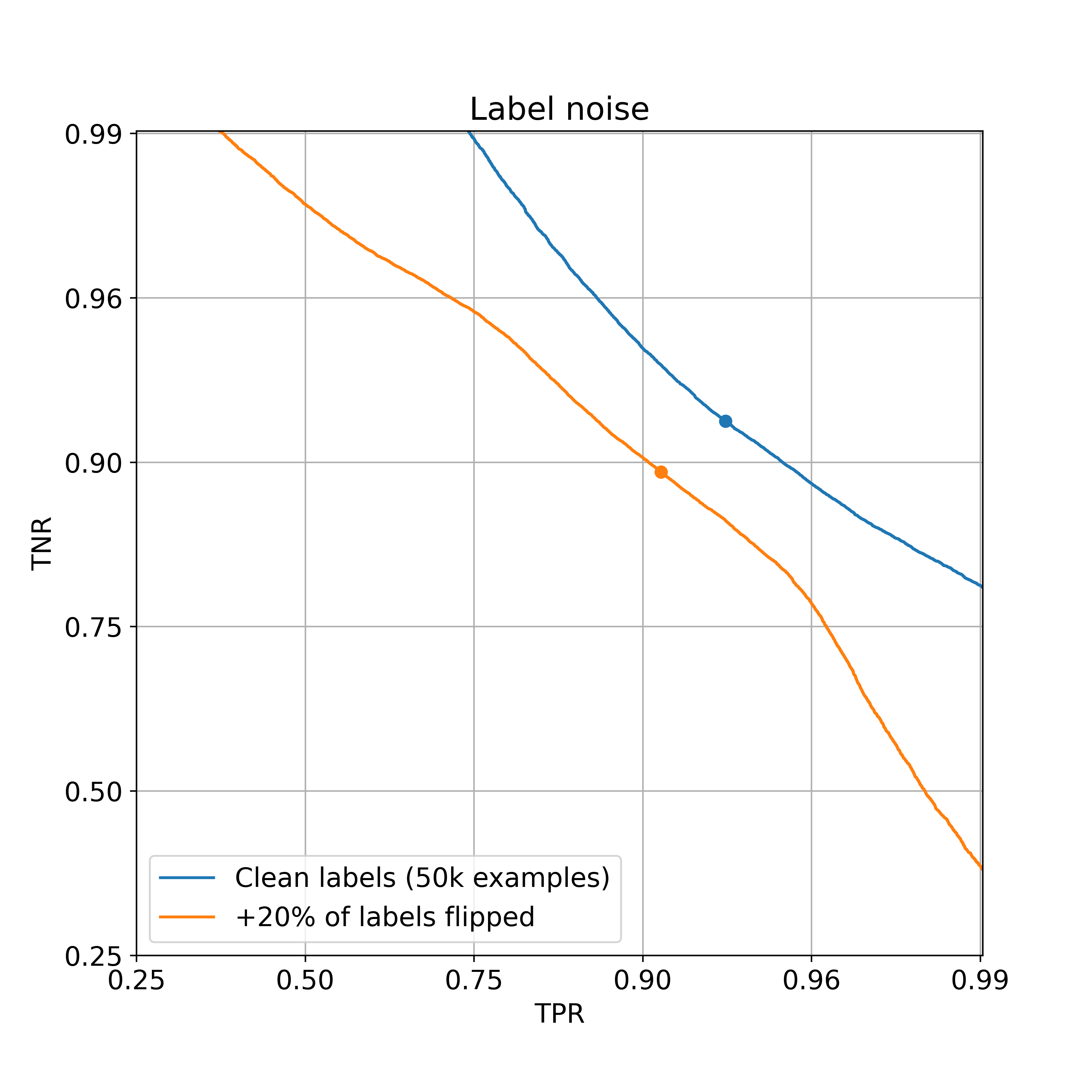
At 99% TPR, the addition of label noise decreases TNR significantly from 76% to 31%. Perhaps this is intuitive: with even a small amount of label noise, there will no longer be any examples on which the model can make a highly confident prediction.
Now let us look at various methods of label cleaning, i.e., selecting a subset of examples to replace the potentially noisy labels with the correct clean ones. We will consider two options, using the model trained on the noisy dataset:
- Select the 10% of examples for which the model’s prediction most disagrees with the given label.
- Select the 10% most confusing examples, without regard for their label.
Applying each of these procedures will generate two new (somewhat cleaner) datasets from the noisy one. Training on these datasets yields the following new ROC curves:
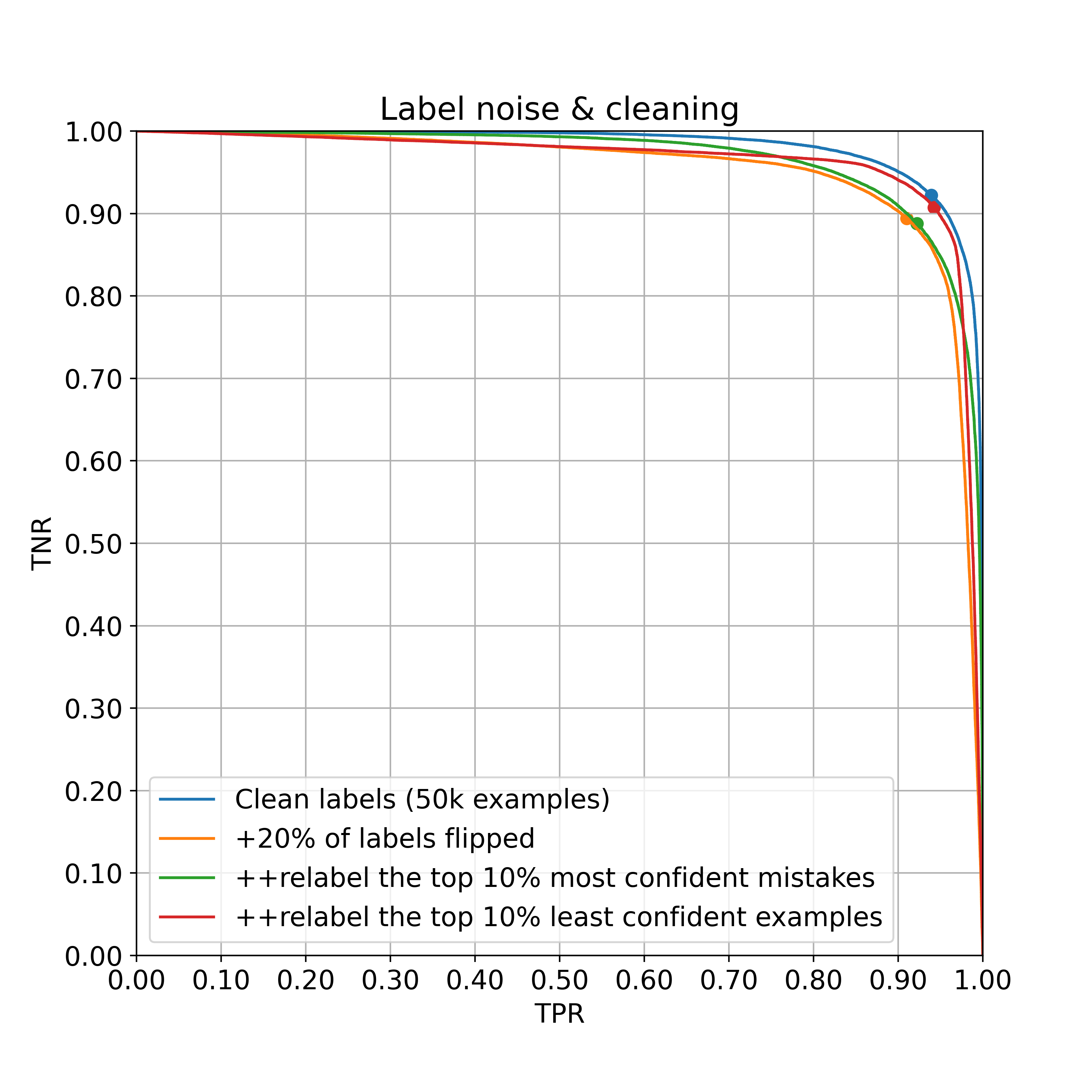
Again, let’s zoom into the top-right 25%.
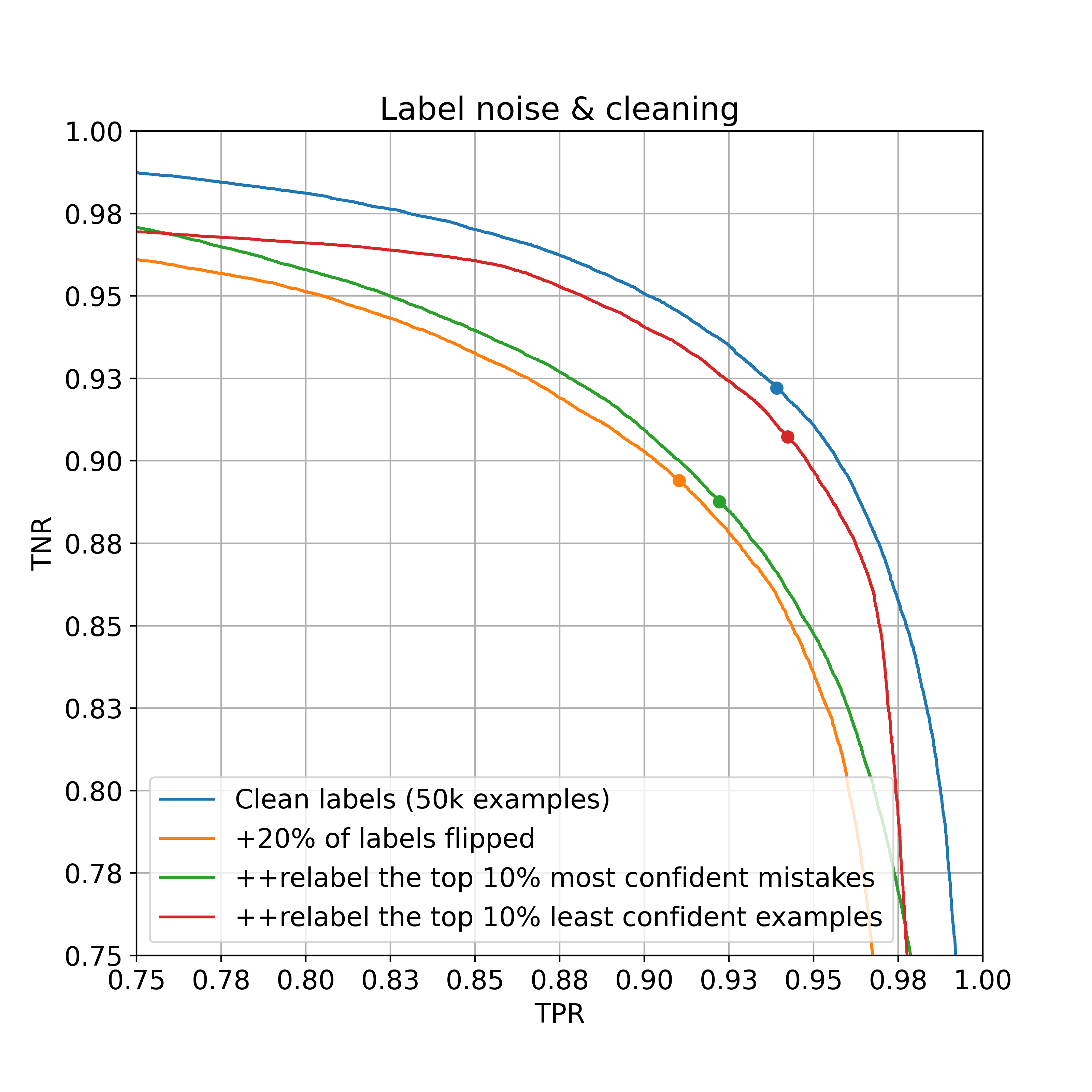
The second strategy is dramatically more effective – relabeling the 10% confident mistakes only boosts balanced accuracy from 90.2% to 90.5%, whereas relabing the 10% most confusing examples boosts to 92.5%. This is surprising, given that the first strategy actually fixes more noisy labels – almost all of the confident mistakes are indeed flipped labels, whereas only around half of confusing examples are.
The result also appears somewhat significant, in that it contradicts common wisdom, which seems to be that fixing these confident mistakes in the dataset are the most important thing to target. (e.g., see the ‘cleanlab’ paper and associated firm)
Ok, but this is only what we saw by zooming into the top-right portion of the ROC curve. Let’s see how things look when we zoom out and use logistic scale in order to more clearly see the high-confidence (high TPR or TNR) regions.
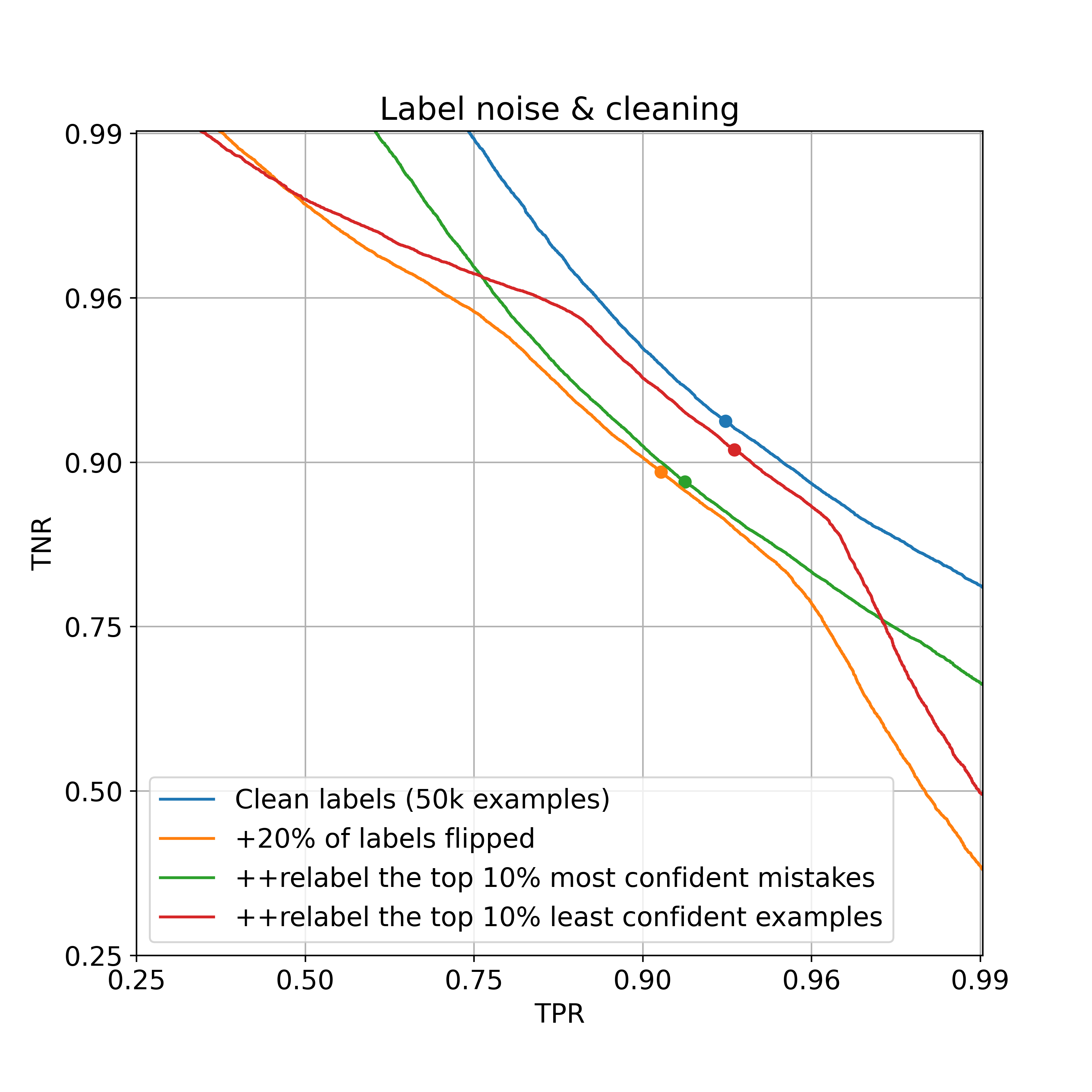
From this wide angle, we can see that strategy 1 actually is useful, for the purpose of improving the model’s behavior in the high-confidence regions of the ROC curve. That is, if we want to maximize accuracy constrained to TPR being 99%, then strategy 1 is most effective. On the other hand, strategy 2 makes almost no difference in these regions. The takeaway is that neither of these strategies is strictly better than the other, rather, each targets a different region of the ROC curve. The better choice ultimately depends upon where we want to operate our model at inference time.
Open question
Is it possible to construct a general theory which predicts the behaviors described in this post?
E.g., does the observation “to max TPR at high TNR, sample positive-heavy” follow from any theory?
I believe that many more such regularities like these can be found, providing a broad empirical basis on which such a theory could be developed. Or maybe such a theory already exists, which I’m not aware of. I would be interested to learn either way.