Muon is an optimizer for the hidden layers in neural networks. It is used in the current training speed records for both NanoGPT and CIFAR-10 speedrunning.
Many empirical results using Muon have already been posted, so this writeup will focus mainly on Muon’s design. First we will define Muon and provide an overview of the empirical results it has achieved so far. Then we will discuss its design in full detail, including connections to prior research and our best understanding of why it works. Finally we will end with a discussion on standards of evidence in optimization research.
Definition
Muon is an optimizer for 2D parameters of neural network hidden layers. It is defined as follows:
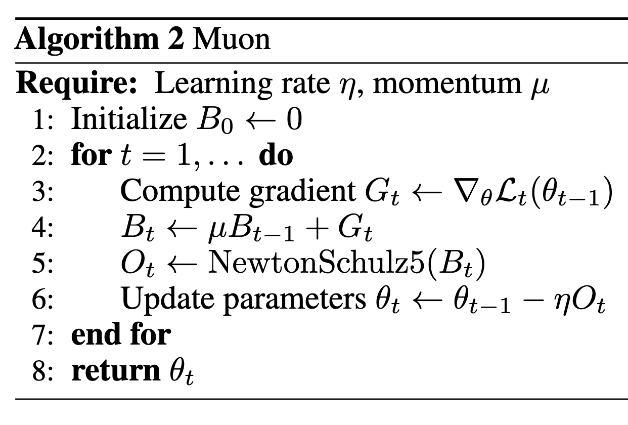
where ‘NewtonSchulz5’ is defined to be the following Newton-Schulz matrix iteration (Bernstein & Newhouse, 2024; Higham, 2008; Björck and Bowie, 1971; Kovarik, 1970):
# Pytorch code
def newtonschulz5(G, steps=5, eps=1e-7):
    assert G.ndim == 2
    a, b, c = (3.4445, -4.7750, 2.0315)
    X = G.bfloat16()
    X /= (X.norm() + eps)
    if G.size(0) > G.size(1):
        X = X.T
    for _ in range(steps):
        A = X @ X.T
        B = b * A + c * A @ A
        X = a * X + B @ X
    if G.size(0) > G.size(1):
        X = X.T
    return X
A ready-to-use PyTorch implementation of Muon can be found here. An example usage in the current NanoGPT speedrun record can be found here.
When training a neural network with Muon, scalar and vector parameters of the network, as well as the input and output layers, should be optimized by a standard method such as AdamW. Muon can be used for 4D convolutional parameters by flattening their last three dimensions (like so).
Results
Muon has achieved the following empirical results.
- Improved the speed record for training to 94% accuracy on CIFAR-10 from 3.3 to 2.6 A100-seconds.
- Improved the speed record for training to 3.28 val loss on FineWeb (a competitive task known as NanoGPT speedrunning) by a factor of 1.35x.
- Continued showing training speed improvements while scaling to 774M and 1.5B parameters.
- Trained a 1.5B parameter transformer to GPT-2 XL level performance on HellaSwag in 10 8xH100-hours. Using AdamW to achieve the same result takes 13.3 hours.
Here’s a comparison between different strong optimizers for NanoGPT speedrunning:
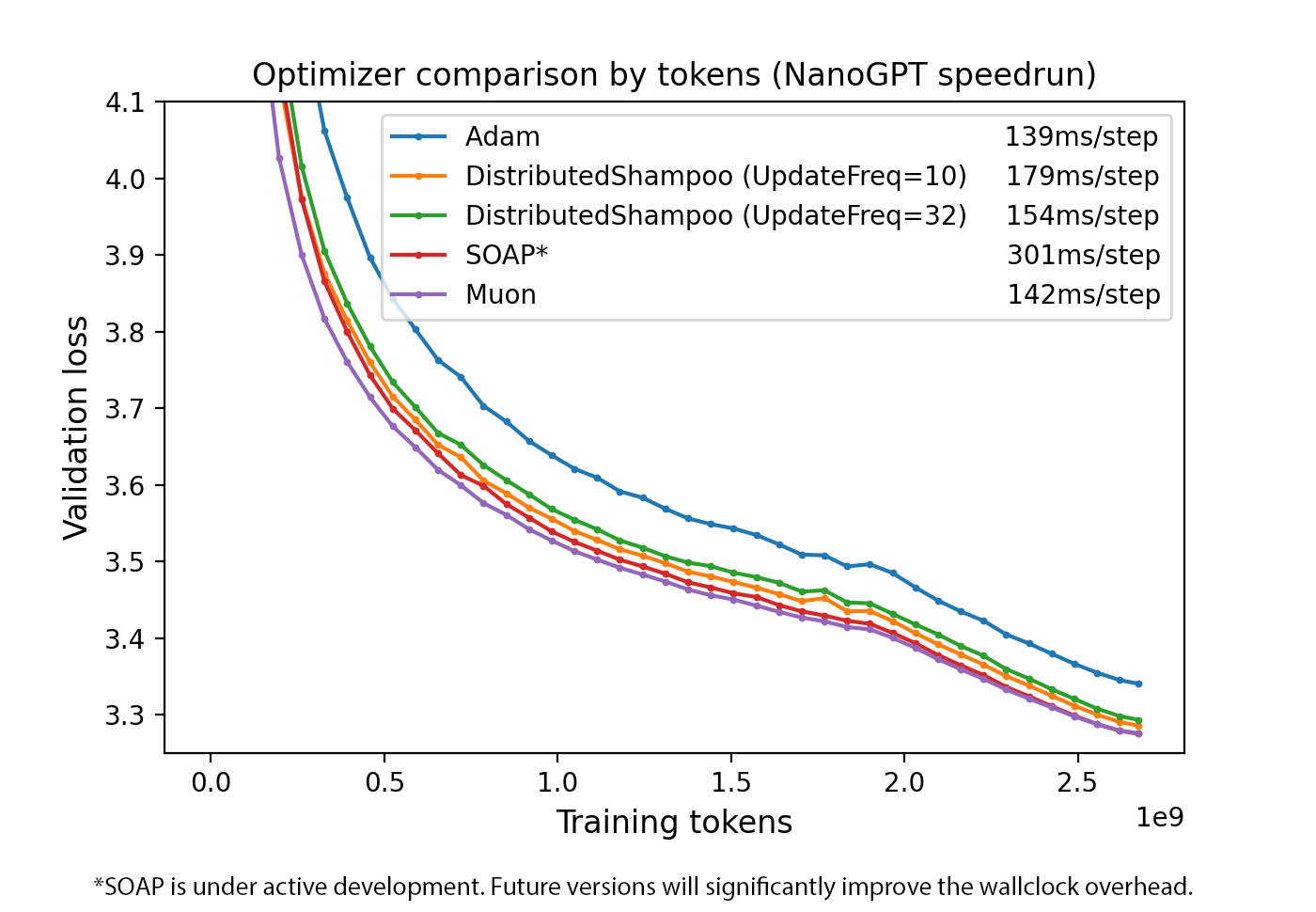 Figure 1. Optimizer comparison by sample efficiency. [reproducible logs]
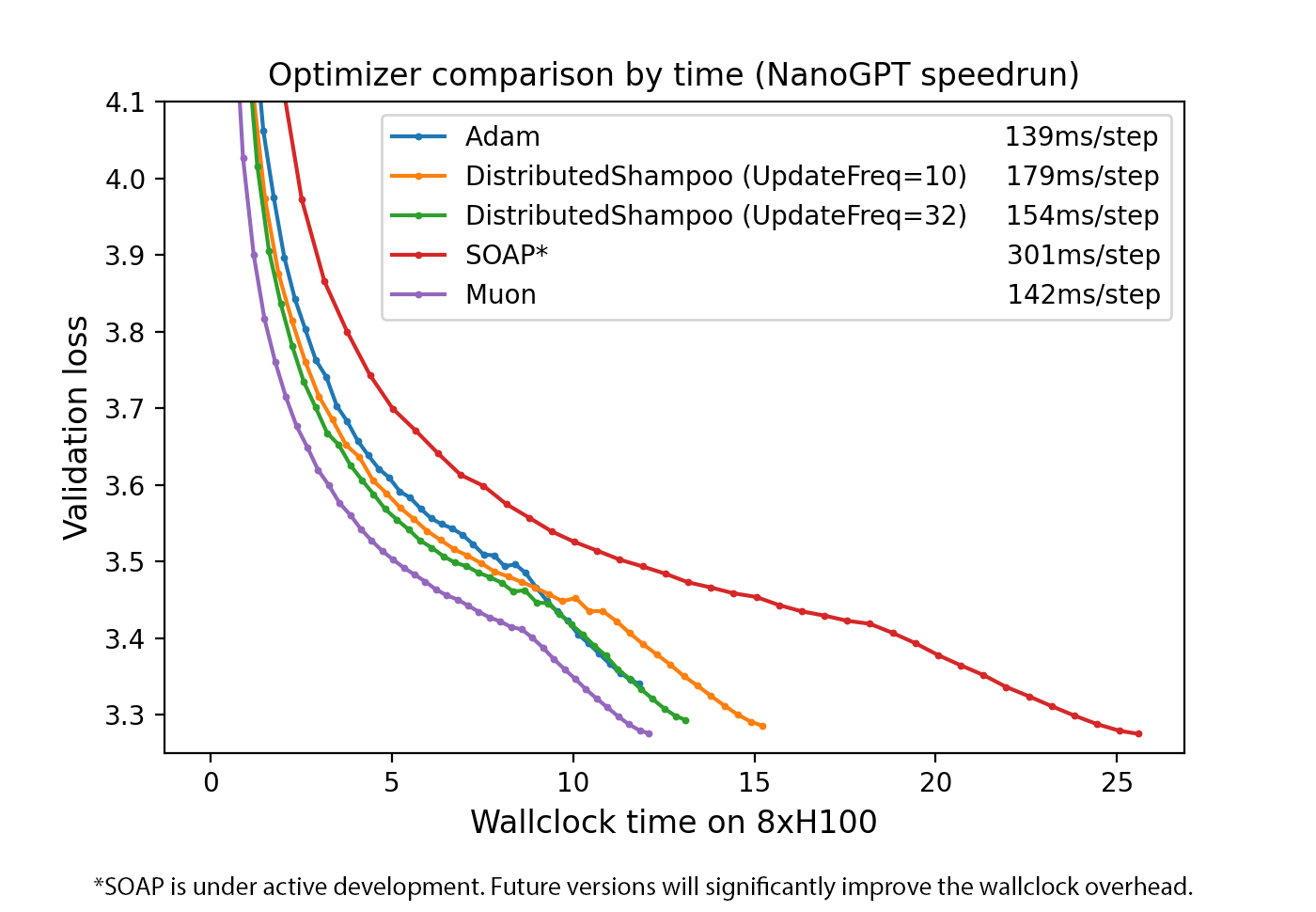 Figure 2. Optimizer comparison by wallclock time.
In addition, here’s a comparison between Muon and AdamW for training a 1.5B-parameter language model.
Both optimizers have been tuned.
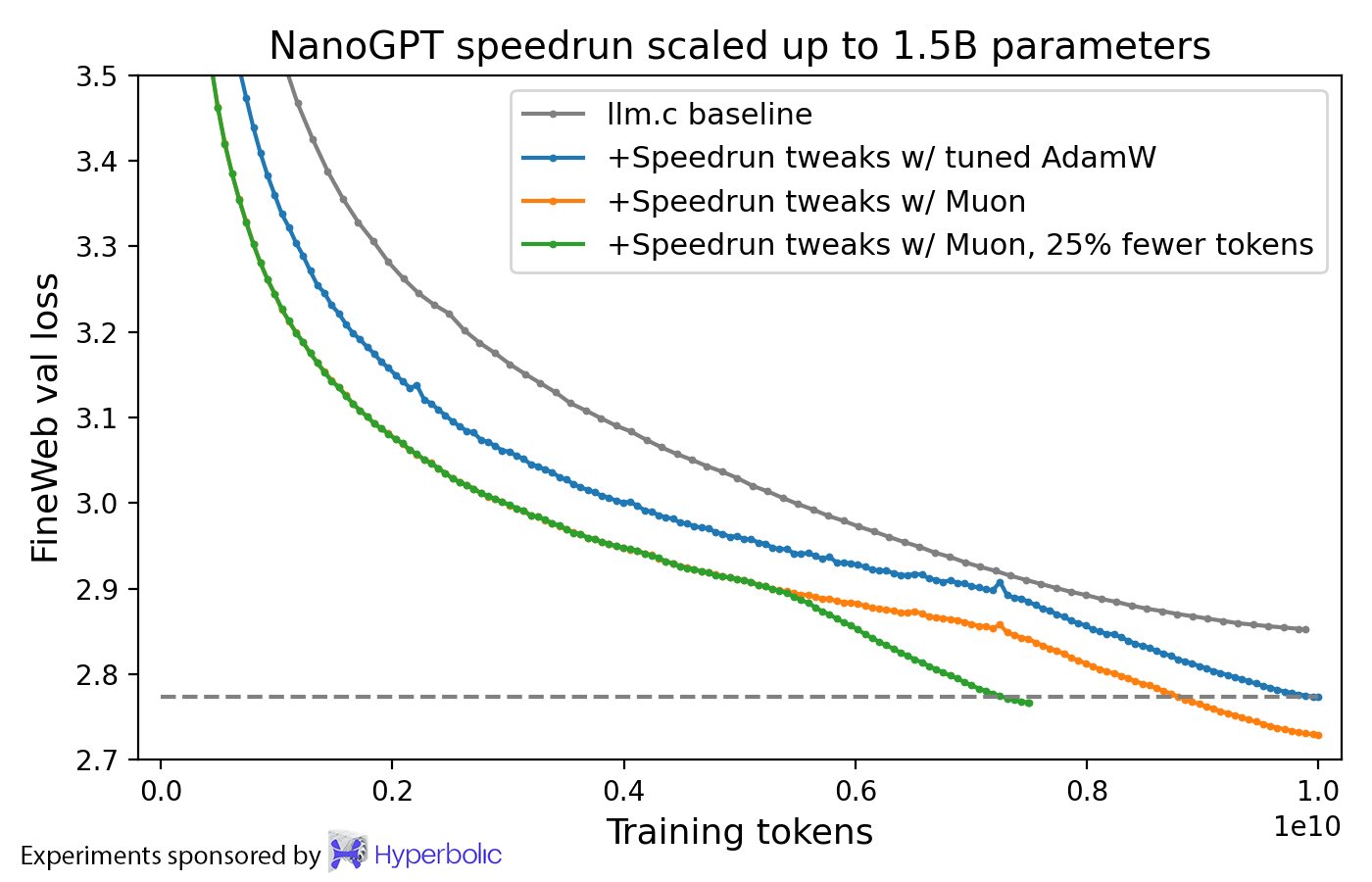 Figure 3. Muon vs. AdamW for a short 1.5B training. [reproducible logs]
The design of Muon
This section describes and analyzes Muon’s design.
Muon (MomentUm Orthogonalized by Newton-Schulz) optimizes 2D neural network parameters by taking the updates generated by SGD-momentum, and then applying a Newton-Schulz (NS) iteration as a post-processing step to each of them before applying them to the parameters.
The function of the NS iteration is to approximately orthogonalize the update matrix, i.e., to apply the following operation:
$$\mathrm{Ortho}(G) = \arg\min_O \{ \|O - G\|_F : \text{either $O^\top O = I$ or $OO^\top = I$} \}$$
In other words, the NS iteration effectively replaces SGD-momentum’s update matrix with the nearest semi-orthogonal matrix to it. This is equivalent to replacing the update by $UV^\top$, where $USV^\top$ is its singular value decomposition (SVD).
Why is it good to orthogonalize the update?
We would first like to observe that one valid answer would be: It just is OK? (Shazeer 2020)

But, for a theoretically-flavored motivation descending from Bernstein & Newhouse (2024)’s analysis of Shampoo (Gupta et al. 2018), see the relationship to Shampoo section.
And for an empirically-flavored motivation, we observe that based on manual inspection, the updates produced by both SGD-momentum and Adam for the 2D parameters in transformer-based neural networks typically have very high condition number. That is, they are almost low-rank matrices, with the updates for all neurons being dominated by just a few directions. We speculate that orthogonalization effectively increases the scale of other “rare directions” which have small magnitude in the update but are nevertheless important for learning.
Eliminating alternatives to NS iteration
There are several other options besides NS iteration for orthogonalizing a matrix. In this subsection I’ll describe why we didn’t use two of them. Please refer to Appendix A of Bernstein & Newhouse (2024) for a more complete list of possible methods.
SVD (i.e., computing the $USV^\top$ decomposition of the update and then replacing the update with $UV^\top$) is easy to understand, but we don’t use it because it’s far too slow.
Coupled Newton iteration (Guo and Higham, 2006; Iannazzo, 2006) is used in implementations of Shampoo (Gupta et al. 2018; Anil et al. 2020; Shi et al., 2023) to perform inverse-fourth roots, and can be easily adapted to perform orthogonalization. But we don’t use it because we find that it must be run in at least float32 precision to avoid numerical instability, which makes it slow on modern GPUs.
In comparison, we find that Newton-Schulz iterations (Bernstein & Newhouse, 2024; Higham, 2008; Björck and Bowie, 1971; Kovarik, 1970) can be stably run in bfloat16. We therefore select them as our method of choice to orthogonalize the update.
Proving that NS iteration orthogonalizes the update
To understand why the NS iteration orthogonalizes the update, let $G = USV^\top$ be the SVD of the update matrix produced by SGD-momentum. Then running one step of the NS iteration with coefficients $(a, b, c)$ yields the following output:
\begin{align*} G’ &:= aG + b(GG^\top)G + c(GG^\top)^2G \\ &= (aI + b(GG^\top) + c(GG^\top)^2)G \\ &= (aI + bUS^2U^\top + cUS^4U^\top)USV^\top \\ &= U(aS + bS^3 + cS^5)V^\top \end{align*}
In general, if we define the quintic polynomial $\varphi(x) = ax + bx^3 + cx^5$, then applying $N$ steps of NS iteration with coefficients $(a, b, c)$ yields the output $U\varphi^N(S)V^\top$, where $\varphi^N(S)$ indicates applying $\varphi$ $N$ times elementwise to the singular values that make up the diagonal of $S$.
As a result, to guarantee that the NS iteration converges to $\mathrm{Ortho}(G) = UV^\top$, all we need to do is (1) ensure that the initial entries of $S$ lie in the range $[0, 1]$, and (2) select the coefficients such that $\varphi^N(x) \to 1$ as $N \to \infty$ for all $x \in [0, 1]$.
To satisfy the first criterion, we simply replace $G$ by $G/\|G\|_F$ before starting the NS iteration. This rescaling is benign because $\mathrm{Ortho}(cG) = \mathrm{Ortho}(G)$.
To satisfy $\varphi^N(x) \to 1$ as $N \to \infty$, we have some freedom, as there are many possible choices of $(a, b, c)$ with this property. Later we will optimize this choice, but for now we show in the below plot that the simple baseline $(a, b, c) = (2, -1.5, 0.5)$ already works.
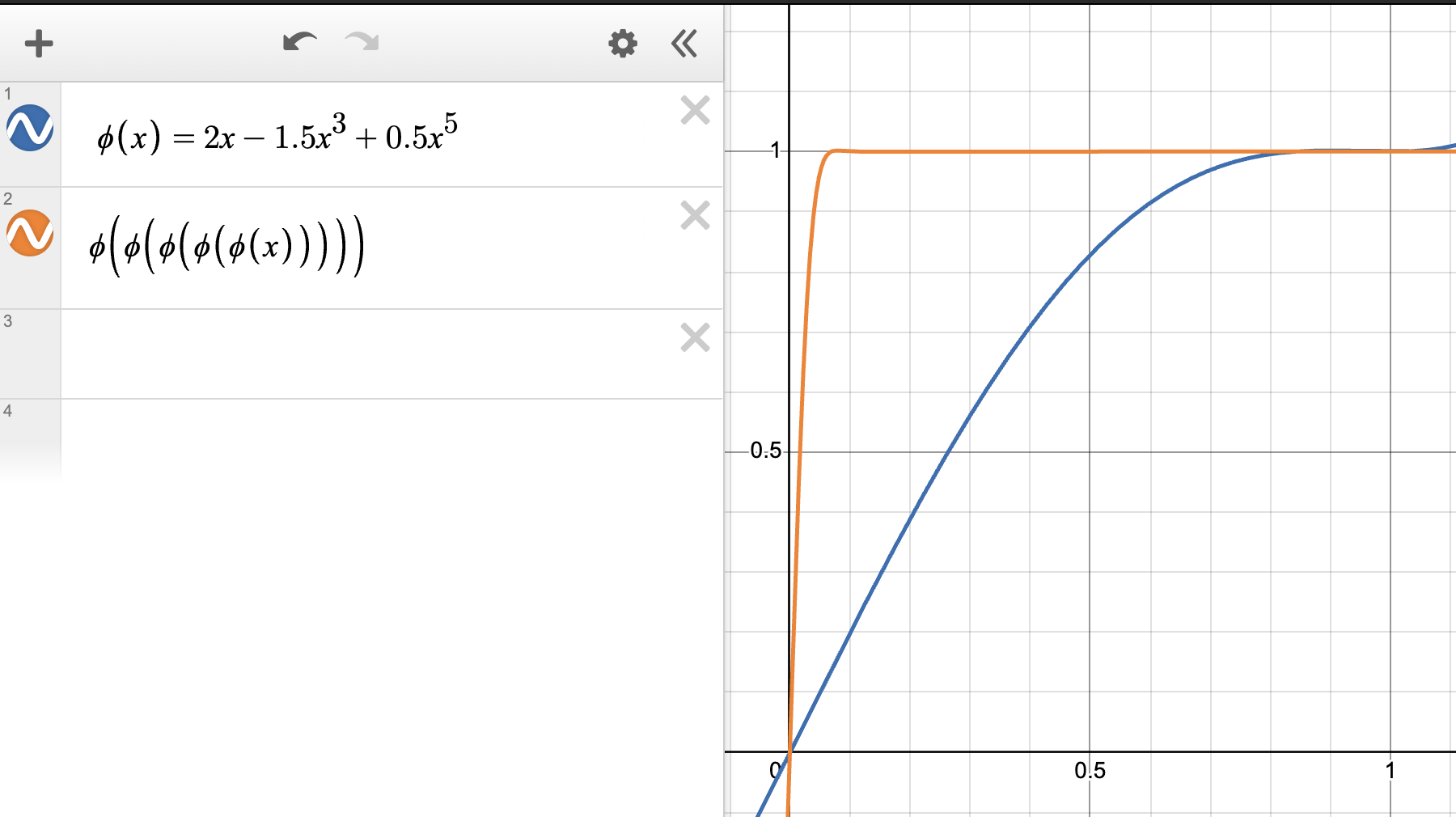 Figure 3. Baseline coefficients for Newton-Schulz iteration.
Tuning the coefficients
Although the NS coefficients $(a, b, c) = (2, -1.5, 0.5)$ work perfectly fine for orthogonalizing the update, they can be further tuned to reduce the number of NS iteration steps we need to run.
For tuning the coefficients $(a, b, c)$, we have the following considerations:
- We want to make $a$ as large as possible, since the fact that $\varphi’(0) = a$ implies that this coefficient is what controls the rate of convergence for small initial singular values.
- For every $x \in [0, 1]$, we want $\varphi^N(x)$ to converge to a value in the range $[1-\varepsilon, 1+\varepsilon]$ as $N \to \infty$, so that the result of the NS iteration is not far from $\mathrm{Ortho}(G)$.
The surprising observation here is that empirically, $\varepsilon$ can be as high as around 0.3 without harming the loss curve for Muon-based trainings. Therefore, our goal will be to maximize $a$ subject to $\lim_{N \to \infty} \varphi^N(x) \in [0.7, 1.3]$.
There are many possible approaches to solve this constrained optimization problem. We use an ad-hoc gradient based approach and end up with the coefficients $(3.4445, -4.7750, 2.0315)$, which is what we use for the final design of Muon. The behavior of these coefficients can be seen in the figure below. Note the steeper growth around x=0.
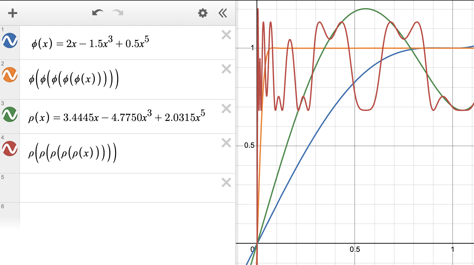 Figure 4. Tuned coefficients for our Newton-Schulz iteration.
In our experiments, when using Muon with these coefficients to train transformer language models and small convolutional networks, it suffices to run the NS iteration for only 5 steps.
We also considered using third-order and seventh-order polynomials for the NS iteration, but found that these could not improve the wallclock overhead any further.
Runtime analysis
In this section we analyze the runtime and memory requirements of Muon.
Before the NS iteration is applied, Muon is just standard SGD-momentum, so it has the same memory requirement.
For each $n \times m$ matrix parameter in the network (w.l.o.g. let $m \leq n$), each step of the NS iteration requires $2(2nm^2 + m^3)$ matmul FLOPs, which is at most $6nm^2$ in the case of a square parameter. Therefore, the extra FLOPs required by Muon compared to SGD is at most $6Tnm^2$, where $T$ is the number of NS iterations (typically we use $T=5$).
If the parameter parametrizes a linear layer, then the baseline amount of FLOPs used to perform a step of training (i.e., a forward and backward pass) is $6nmB$, where $B$ is the number of inputs passed through the layer during the step.
Therefore, the FLOP overhead of Muon is at most $Tm/B$, where $m$ is the model dimension, $B$ is the batch size in tokens, and $T$ is the number of NS iteration steps (typically $T=5$).
We now calculate this overhead for two concrete training scenarios: NanoGPT speedrunning, and Llama 405B training.
- For the current NanoGPT speedrunning record, the model dimension is $m=768$, and the number of tokens per batch is $B=524288$. Therefore, the overhead is $5*768/524288 = 0.7\%$.
- For Llama 405B training, the model dimension is $m=16384$ And the number of tokens per batch is reported to be $B=16000000$ (Dubey et al. 2024). Therefore, the overhead of using Muon for this training would be $5*16384/16000000 = 0.5\%$.
We conclude that for typical LM training scenarios, at both the small and large scale, Muon has a FLOP overhead below 1%.
Relationship to prior optimizers
Shampoo
The Shampoo optimizer is defined as follows (Gupta et al. 2018).
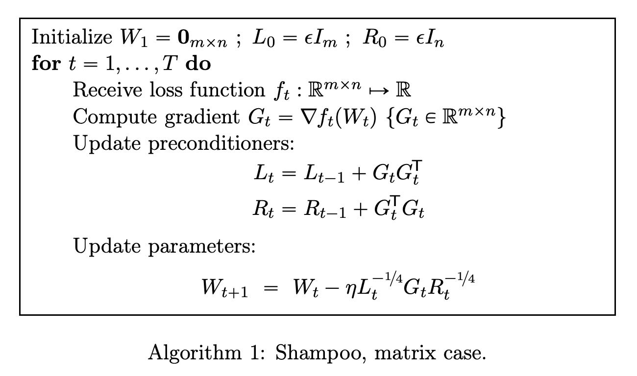
If preconditioner accumulation is removed, then Bernstein & Newhouse (2024) observed that the update becomes the following (also see Anil (2024a)): \begin{align*} W_{t+1} &= W_t - \eta (G_tG_t^\top)^{-1/4}G_t(G_t^\top G_t)^{-1/4} \\ &= W_t - \eta (US^2U^\top)^{-1/4} (USV^\top) (VS^2V^\top)^{-1/4} \\ &= W_t - \eta (US^{-1/2}U^\top) (USV^\top) (VS^{-1/2}V^\top) \\ &= W_t - \eta US^{-1/2}SS^{-1/2}V^\top \\ &= W_t - \eta UV^\top \end{align*}
Which is the orthogonalized gradient. If we then add momentum before the orthogonalization, we recover the Muon update, albeit with a higher wallclock and FLOP overhead due to the usage of inverse-fourth roots rather than Newton-Schulz iteration.
It is therefore possible to interpret Muon with momentum turned off as a kind of “instantaneous" or “accumulation-free” Shampoo (Anil 2024b).
Orthogonal-SGDM
Tuddenham et al. (2022) proposed to optimize neural networks by orthogonalizing the gradient via SVD, applying momentum to the result, and then using the momentum term as the update, calling this optimizer Orthogonal-SGDM. This is similar to Muon, with the difference being that Muon moves the momentum to before the orthogonalization, which we find performs better empirically, and uses a Newton-Schulz iteration instead of SVD for more efficient orthogonalization. In their best-performing experimental setup (Table 3), Tuddenham et al. (2022) reported that their method is outperformed by a well-tuned standard SGD-Momentum, which perhaps accounts for the fact that this paper was not cited prior to this blogpost.
Stochastic spectral descent and RMSspectral
Note: This subsection was added on 07/12/2025.
Yet an earlier example of orthogonalization-based optimization can be found in the work of Carlson et al. (2015a, 2016), who proposed to optimize restricted Boltzmann machines and discrete graphical models by orthogonalizing their gradient estimates using SVD and then scaling by the nuclear norm, calling this method stochastic spectral descent. In addition, Carlson et al. (2015b) proposed to optimize feedforward neural networks using a hybrid between stochastic spectral descent and RMSprop, called RMSspectral. Anticipating the need to speed up orthogonalization, RMSspectral uses randomized SVD instead of full SVD to approximate the orthogonalization operation. Compared to Muon, these pioneering early orthogonalization-based optimizers use SVD variants instead of Newton-Schulz iteration for orthogonalization, and lack any form of momentum. We find that using momentum is necessary for the best empirical performance.
Empirical considerations
By design, Muon only applies to 2D parameters (and convolutional filters via flattening), so the remaining scalar and vector parameters in a network must be optimized using a standard method (e.g., AdamW). Empirically, we find that it is also important to optimize input and output parameters using AdamW, even though these are typically 2D. In particular, when training transformers, AdamW should be used for the embedding and final classifier head layers in order to attain the best performance. That the optimization dynamics of the embedding layer should be different from other layers follows from the modular norm theory (Large et al. 2024). That such dynamics are also different for the output layer does not seem to follow from the theory, and is instead driven by empirics.
Another purely empirical result is that using Nesterov-style momentum for Muon works a bit better than normal SGD-momentum in every case we have tested. We have therefore made this the default in the public Muon implementation.
A third result is that Muon works better for optimizing transformers if it is applied to their Q, K, V parameters separately, rather than together as would be the default for transformer implementations that parametrize QKV as a single linear layer whose outputs are split.
Discussion: Solving the undertuned baseline problem with the competitive task framework
The neural network optimization research literature is by now mostly filled with a graveyard of dead optimizers that claimed to beat AdamW, often by huge margins, but then were never adopted by the community. Hot take, I know.
With billions of dollars being spent on neural network training by an industry hungry for ways to reduce that cost, we can infer that the fault lies with the research community rather than the potential adopters. That is, something is going wrong with the research. Upon close inspection of individual papers, one finds that the most common culprit is bad baselines: Papers often don’t sufficiently tune their AdamW baseline before comparing it to a newly proposed optimizer.
I would like to note that the publication of new methods which claim huge improvements but fail to replicate / live up to the hype is not a victimless crime, because it wastes the time, money, and morale of a large number of individual researchers and small labs who run and are disappointed by failed attempts to replicate and build on such methods every day.
To remedy this situation, I propose that the following evidential standard be adopted: The research community should demand that, whenever possible, new methods for neural network training should demonstrate success in a competitive training task.
Competitive tasks solve the undertuned baseline problem in two ways. First, the baseline in a competitive task is the prior record, which, if the task is popular, is likely to already be well-tuned. Second, even in the unlikely event that the prior record was not well-tuned, self-correction can occur via a new record that reverts the training to standard methods. The reason this should be possible is because standard methods usually have fast hardware-optimized implementations available, whereas new methods typically introduce some extra wallclock overhead; hence simply dropping the newly proposed method will suffice to set a new record. As a result, the chance of a large but spurious improvement to a standard method being persistently represented in the record history for a popular competitive task is small.
To give an example, I will describe the current evidence for Muon. The main evidence for it being better than AdamW comes from its success in the competitive task “NanoGPT speedrunning.” In particular, switching from AdamW to Muon set a new NanoGPT training speed record on 10/15/24, where Muon improved the training speed by 35%. Muon has persisted as the optimizer of choice through all 12 of the new NanoGPT speedrunning records since then, which have been set by 7 different researchers.
Muon has a slower per-step wallclock time than AdamW, so if there existed hyperparameters that could make AdamW as sample-efficient as Muon, then it would be possible to set a new record by simply chucking Muon out of the window and putting good old AdamW back in. Therefore, to trust that Muon is better than AdamW, at least for training small language models, you actually don’t need to trust me (Keller Jordan) at all. Instead, you only need to trust that there exist researchers in the community who know how to tune AdamW and are interested in setting a new NanoGPT speedrunning record. Isn’t that beautiful?
Remaining open questions
- Will Muon scale to larger trainings? (e.g., 20B+ parameters for 1T+ tokens)
- Will it be possible to properly distribute the Newton-Schulz iterations used by Muon across a large-scale GPU cluster?
- Is it possible that Muon works only for pretraining, and won’t work for finetuning or reinforcement learning workloads?
At the time of writing, I don’t know the answers to these questions.
Muon Contributors
The following researchers have made contributions to Muon.
- Jeremy Bernstein & Laker Newhouse sent me their paper Old Optimizer, New Norm: An Anthology, which in Appendix A recommends Newton-Schulz iteration as a computational strategy for Shampoo. Jeremy had also been posting theories on X about a closely related algorithm called steepest descent under spectral norm for several months prior to the development & demonstration of Muon. Lastly, Jeremy helped by pointing out that the coefficients of an earlier version of my NS iteration could be further tuned.
- Vlado Boza showed experimentally the result that Muon works better when applied separately to the Q,K,V parameters, instead of joining them into one matrix.
- Yuchen Jin performed experiments demonstrating that Muon training scales to longer durations and larger models. And he provided the majority of the necessary capital (in H100-hours) for the project.
- Jeremy Bernstein, Jiacheng You, and Franz Cesista discovered that the efficiency of my initial Newton-Schulz iteration implementation could be improved from $6nm^2$ to $4nm^2 + 2m^3$ FLOPs (for a parameter of shape $n \times m$ where $m \leq n$). Jeremy Bernstein and Jiacheng You concurrently discovered the better variant and Franz Cesista made a pull request to the speedrunning repository benchmarking and implementing it.
References
- Vineet Gupta, Tomer Koren, and Yoram Singer. “Shampoo: Preconditioned stochastic tensor optimization.” International Conference on Machine Learning. PMLR, 2018.
- Jeremy Bernstein and Laker Newhouse. “Old optimizer, new norm: An anthology.” arXiv preprint arXiv:2409.20325 (2024).
- Keller Jordan, Jeremy Bernstein, Brendan Rappazzo, @fernbear.bsky.social, Boza Vlado, Jiacheng You, Franz Cesista, Braden Koszarsky, and @Grad62304977. modded-nanogpt: Speedrunning the NanoGPT baseline. 2024. Available at: https://github.com/KellerJordan/modded-nanogpt.
- Rohan Anil et al. “Scalable second order optimization for deep learning.” arXiv preprint arXiv:2002.09018 (2020).
- Rohan Anil. “Just some fun linear algebra.” X post, 6 Oct. 2024, Available at: https://x.com/_arohan_/status/1843050297985466565.
- Rohan Anil. “Shampoo with no accumulation ❤️.” X post, 20 Oct. 2024, Available at: https://x.com/_arohan_/status/1848065162919448889.
- Abhimanyu Dubey et al. “The llama 3 herd of models.” arXiv preprint arXiv:2407.21783 (2024).
- C.-H. Guo and N. J. Higham. A Schur-Newton method for the matrix p’th root and its inverse. SIAM Journal On Matrix Analysis and Applications, 28(3):788–804, 2006.
- B. Iannazzo. On the Newton method for the matrix p-th root. SIAM journal on matrix analysis and applications, 28(2):503–523, 2006.
- Andrej Karpathy. nanoGPT: The simplest, fastest repository for training/finetuning medium-sized GPTs. GitHub repository, 2023. Available at: https://github.com/karpathy/nanoGPT.
- Tim Large et al. “Scalable Optimization in the Modular Norm.” arXiv preprint arXiv:2405.14813 (2024).
- Hao-Jun Michael Shi et al. “A distributed data-parallel pytorch implementation of the distributed shampoo optimizer for training neural networks at-scale.” arXiv preprint arXiv:2309.06497 (2023).
- Nicholas J. Higham. Functions of Matrices. Society for Industrial and Applied Mathematics, 2008.
- Zdislav Kovarik. Some iterative methods for improving orthonormality. SIAM Journal on Numerical Analysis, 1970.
- Åke Björck and C. Bowie. An iterative algorithm for computing the best estimate of an orthogonal matrix. SIAM Journal on Numerical Analysis, 1971.
- Noam Shazeer. “Glu variants improve transformer.” arXiv preprint arXiv:2002.05202 (2020).
- Jeremy Cohen et al. “Understanding Optimization in Deep Learning with Central Flows.” arXiv preprint arXiv:2410.24206 (2024).
- Mark Tuddenham, Adam Prügel-Bennett, and Jonathan Hare. “Orthogonalising gradients to speed up neural network optimisation.” arXiv preprint arXiv:2202.07052 (2022).
- Keller Jordan. “The new optimizer is defined as follows. It is based on orthogonalizing the update given by SGD-Nesterov-momentum in an efficient way.” X.com snapshot https://archive.is/RZYBG. (Oct 4 2024).
- Ben Recht. “Too Much Information.” Blog post https://www.argmin.net/p/too-much-information#:~:text=benchmark%20competitions%20are%20the%20prime%20mover%20of%20AI%20progress. (Dec 19 2023)
- David Carlson, Volkan Cevher, and Lawrence Carin. Stochastic spectral descent for Restricted Boltzmann Machines. In International Conference on Artificial Intelligence and Statistics, 2015a.
- David Carlson, Edo Collins, Ya-Ping Hsieh, Lawrence Carin, and Volkan Cevher. Preconditioned spectral descent for deep learning. In Neural Information Processing Systems, 2015b.
- David Carlson, Ya-Ping Hsieh, Edo Collins, Lawrence Carin, and Volkan Cevher. Stochastic spectral descent for discrete graphical models. Selected Topics in Signal Processing, 2016.
Citation
@misc{jordan2024muon,
  author       = {Keller Jordan and Yuchen Jin and Vlado Boza and Jiacheng You and
                  Franz Cesista and Laker Newhouse and Jeremy Bernstein},
  title        = {Muon: An optimizer for hidden layers in neural networks},
  year         = {2024},
  url          = {https://kellerjordan.github.io/posts/muon/}
}