In this post we explore a second empirical law of neural network training, this time regarding the influence of training data.
The main result is that, if we get rid of the inherent noise in the training process by averaging over many repeated runs, then the effect of each additional training example is approximately additive.
Setup
For a machine learning problem where the goal is to map inputs from a space $\mathcal X$ to $k$ real-valued outputs, we call functions of the form $f: \mathcal X \to \mathbb R^k$ hypotheses. For example, neural networks trained on CIFAR-10 compute hypotheses of the form $\mathbb R^{32 \times 32 \times 3} \to \mathbb R^{10}$. We denote the space of all hypotheses for the problem by $\mathcal H := \{f: \mathcal X \to \mathbb R^k\}$.
Training neural networks is an inherently stochastic process, as evidenced by the fact that varying just a single parameter at initialization induces nearly the same amount of inter-run variance by the end of training as does a fully random initialization (Summers et al. 2021, Jordan 2023). Therefore, there is no meaningful way to reduce the variance of neural network training, besides arbitrarily picking a value at which to fix the random seed.
Because of this fact, in this paper we mathematically model neural network trainings as generating distributions over hypotheses, rather than a specific hypothesis per hyperparameter setting. If $\mathcal A$ denotes a neural network training with fixed hyperparameters (e.g., this one), then we write $f \sim \mathcal H_{\mathcal A}$ to denote that $f$ is a hypothesis sampled from the probability distribution of all hypotheses which can be produced by running $\mathcal A$. Sampling from the distribution $f \sim \mathcal H_{\mathcal A}$ is as simple as running the training and collecting the resulting network.
For a given training $\mathcal A$, we define its mean hypothesis $\bar f_{\mathcal A} \in \mathcal H$ as being the hypothesis $\bar f_{\mathcal A}(x) := \mathbb E_{f \sim \mathcal H_{\mathcal A}}[f(x)]$. Note that the outputs of $\bar f_{\mathcal A}$ are equal to the average outputs from an ensemble of independently trained networks, in the limit as the size of the ensemble goes to infinity.
If $f \sim \mathcal H_{\mathcal A}$, and we define $\varepsilon_f := f - \bar f_{\mathcal A}$, then we have $\mathbb E[\varepsilon_f] = 0$. Therefore, our understanding of neural network training is that every run produces a hypothesis $f$ given by the mean hypothesis $\bar f_{\mathcal A}$, plus an inter-run hypothesis-noise term $\varepsilon_f$. That is: \begin{equation} f = \bar f_{\mathcal A} + \varepsilon_f. \end{equation}
We are interested in understanding the effect of various hyperparameters on the outcome of neural network training. In this post (and the previous one) we study the how $\bar f_{\mathcal A}$ changes as we change various hyperparameters of $\mathcal A$. The benefit of studying $\bar f_{\mathcal A}$ rather than the individual neural networks $f = \bar f_{\mathcal A} + \varepsilon_f$ is that, as we will show, $\bar f_{\mathcal A}$ has much more lawful empirical behavior.
In this post we experiment with a single CIFAR-10 training configuration (this one, which descends from the CIFAR-10 speed record) and vary the training dataset.
To simplify notation, we write $\bar f_{S’}$ to denote the mean hypothesis generated by running the training algorithm with training data $S’$.
Main Experiment
We demonstrate that when $A, B$ are two random large subsets of CIFAR-10, then the following formula holds.
Equation 1. \begin{equation} \bar f_{A \cup B} \approx \bar f_A + \bar f_B - \bar f_{A \cap B}. \end{equation}
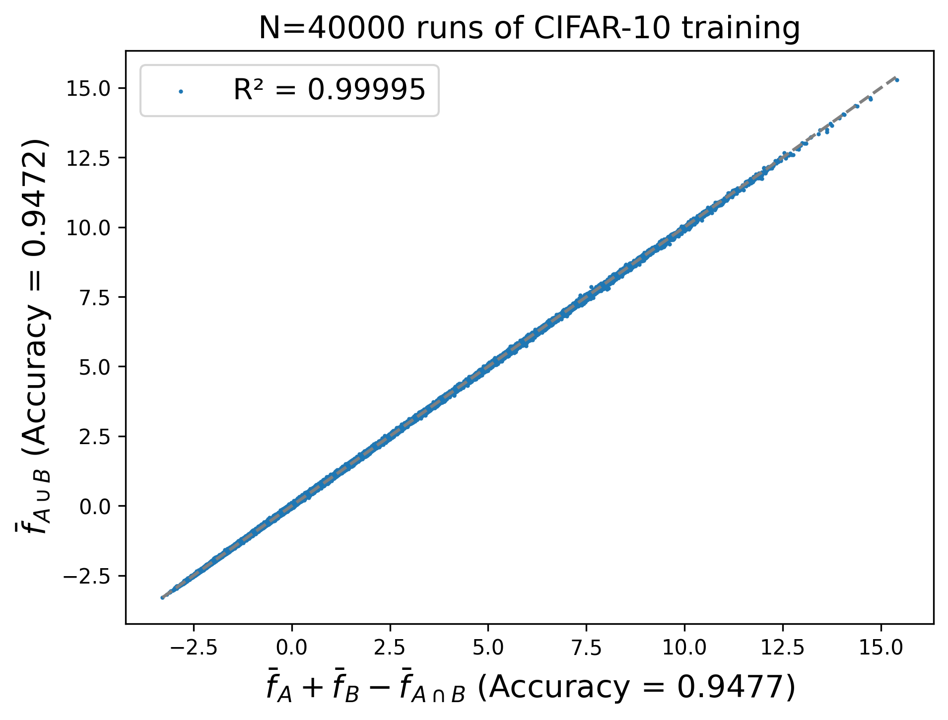
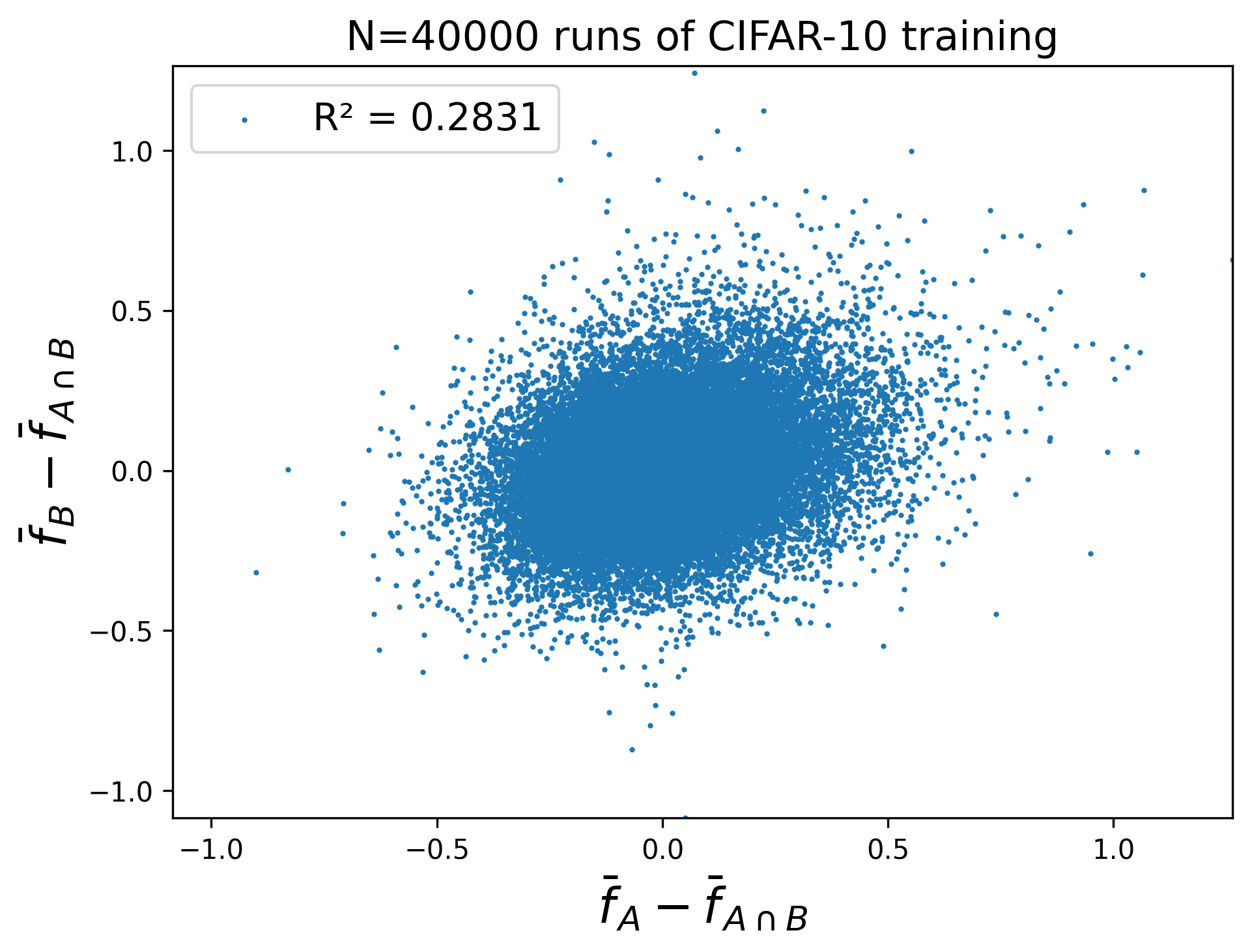
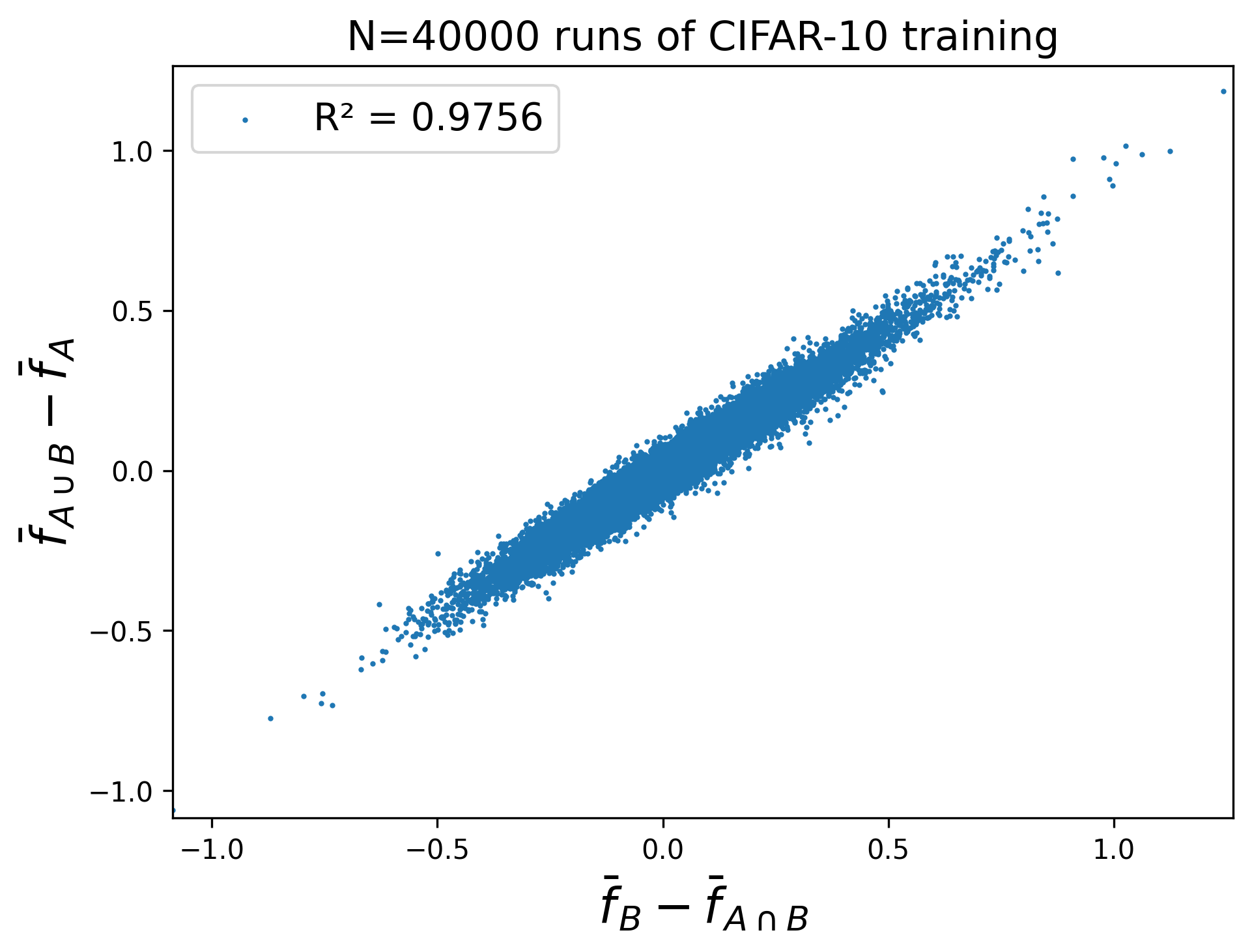
Figure 1. Training data has a locally additive influence on the mean hypothesis.
In Figure 1, we test this figure wiht $A$ being the first 45K CIFAR-10 training examples, and $B$ the first 40K plus the last 5K. Thus $A \cap B$ is the first 40K examples, and $A \cup B$ is the entire set of 50K examples. We find that the formula holds with a high degree of accuracy.
Our real motivation leading to this result was simply to search for empirical laws. But it can also be motivated from a ‘federated-learning’ perspective:
Suppose that we have two training dataset $A$ and $B$, with some overlap. Ideally we would like to train on their union $A \cup B$ to get the best result. But suppose that we are not allowed to do this (perhaps due to privacy concerns). Instead, we are only allowed to train models on $A$ or $B$ individually (or any subsets thereof).
Then our question is: How can we combine the resulting models to recover the performance of training on $A \cup B$ ?
Figure 1 shows that if we are training ensembles, the correct thing to do is use $g(x) := \bar f_A(x) + \bar f_B(x) - \bar f_{A \cup B}(x)$. To show that this is a nontrivial result, let’s compare it to the naive approach of just ensembling $\bar f_A$ and $\bar f_B$.
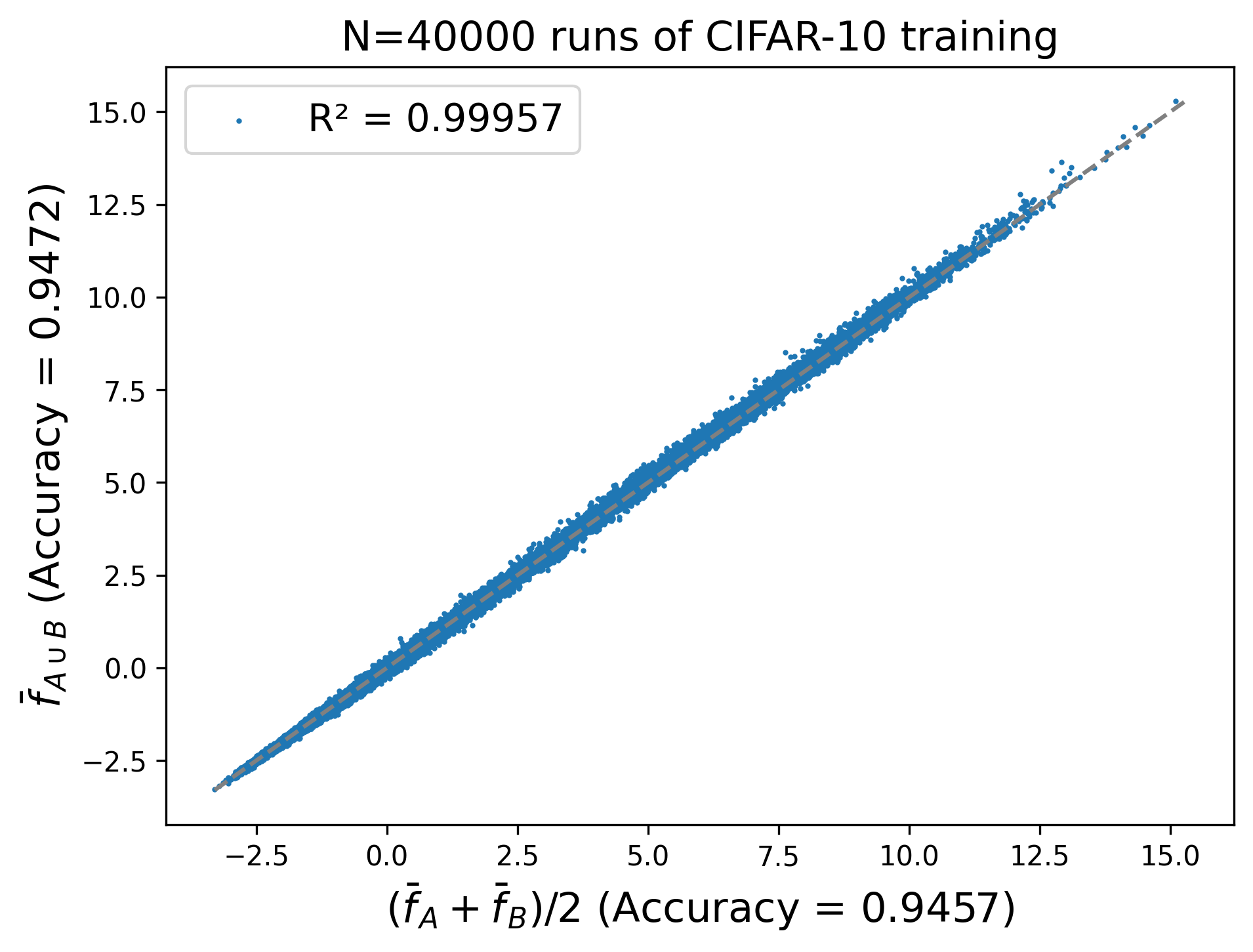 Figure 2. Naive federated ensembling is suboptimal.
We can see that this method of federated ensembling leaves almost 10x more unexplained variance than the correct formula (Figure 1). It also loses 0.17% accuracy compared to $\bar f_{A \cup B}$, whereas Formula 1 loses none.
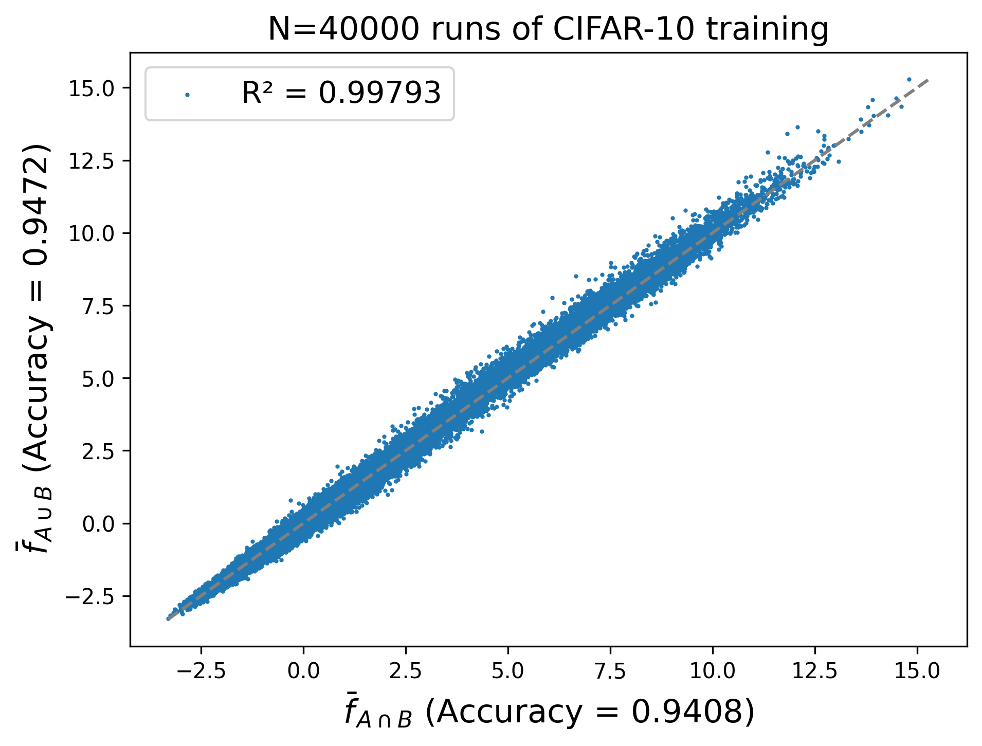
For the sake of completeness, we also try using $\bar f_{A \cap B}$, which is around another order of magnitude worse in terms of $R^2$.
Local Additivity
Definition
Definition 1. We say that a stochastic training algorithm $\mathcal A$ satisifes local additivity over a training dataset $S = ((x_1, y_1), \dots, (x_n, y_n))$ relative to a base dataset $D$ if there exists a set of hypotheses $\bar f_1, \dots, \bar f_n \in \mathcal H$ such that \begin{equation} \bar f_{D \sqcup S’} = \bar f_D + \sum_{i=1}^n \bar f_i \cdot 1\{(x_i, y_i) \in S’\} \end{equation} for every subset $S’ \subseteq S$.
Local additivity is equivalent to the statement that Equation 1 holds across a certain class of dataset pairs.
Theorem 1. The following two statements are equivalent:
If $A, B$ is any pair of datasets such that $(A \cup B) \subseteq (D \cup S)$ and $(A \cap B) \supseteq D$, then $\bar f_{A \cup B} = \bar f_A + \bar f_B - \bar f_{A \cap B}$.
$\mathcal A$ is locally additive over $S$ relative to $D$.
Proof in Appendix.
Result 1: Neural network training is not locally additive relative to $D = \varnothing$.
Comment: The global addivity assumption of Ilyas et al. (2022) would imply that $\mathcal A$ satisfies local additivity over all $S, D$ pairs.
Corollary: Global additivity is wrong.
Neural network training satisfies local additivity when the base dataset is large and random
Discussion
My presentation so far has been light on motivation. Let me explain what motivated the formula $\bar f_A + \bar f_B - \bar f_{A \cap B}$.
Related Work: Globally Linear Datamodeling
In Datamodels: Predicting Predictions from Training Data, Ilyas et al. (2022) proposed to model the influence of data on the mean hypothesis as being globally linear. In particular, they propose that for every input $x$, there exist datamodel weights $\theta_1, \dots, \theta_n$ such that $\bar f_{S’}(x)$ can be approximated as a linear function of $S’ \subseteq S$: \begin{equation} \bar f_{S’}(x) \approx \theta^T 1_{S’} \end{equation} where $1_{S’} \in \{0, 1\}^n$ is defined as the indicator vector for the subset $S’$, so that $\theta^T 1_{S’} = \sum_{i=1}^n \theta_i \cdot 1\{(x_i, y_i) \in S’\}$.
To estimate these weights, they sample a series of random training subsets $S_1’, \dots, S_m’ \subseteq S$, and then optimize $\theta$ to minimize the following cost function \begin{equation} \mathcal L(\theta) = \frac1m \sum_{j=1}^m (\theta^T 1_{S_j’} - \bar f_{S_j’}(x))^2 + \lambda |w|_1 \end{equation} where the mean hypotheses $\bar f_{S’}(x)$ are noisily estimated by a single run of training per subset, across hundreds of thousands of random subsets. The estimated datamodel weights enable several remarkable applications, including duplicate detection and estimation of data support size for each test example.
The estimated datamodel weights enable several remarkable demonstrations. First, Ilyas et al. (2022) show that for around half of CIFAR-10 test examples, there exists a set of 250 training examples whose removal from the training set causes the test example to be misclassified. They locate such sets using the maximum datamodel weights. Second, the datamodels can be used as high-quality feature embeddings, enabling duplicate detection.To demonstrate the predictiveness of the estimated datamodel weights, Ilyas et al. (2022) compare the predictions $\theta^T 1_{S’}$ to the ground truth mean hypotheses $\bar f_{S’}(x)$, across hundreds of new random subsets $S’ \subseteq S$ which were not used in the optimization process. For this comparison, the mean hypotheses are estimated using 100 runs of training per subset.
Based on our digitization of the provided figure (Figure 5 in Ilyas et al. (2022)), we observe that at the level of individual examples, the Pearson correlation between the linear datamodel predictions $\theta^T 1_{S’}$ and the ground truth $\bar f_{S’}(x)$ is between 0.8 and 0.9 for most examples, indicating that linear datamodeling is indeed able to at least partially model the influence of data on neural network training. We conclude that there is still a substantial gap between the approximation of data influence provided by linear datamodels and the ground truth reality.
Footnote: The loss function minimized by Ilyas et al. (2022) differs from Equation 2 in two senses. First, the authors do not model the behavior of the mean hypothesis, but rather the behavior of individual networks generated by training. This yields a mathematically equivalent but noisier loss function. Second, the authors model the correct-class margin of a test example $(x, y)$, rather than the logit outputs on $x$, causing their datamodel weight to have shape $w \in \mathbb R^n$ compared to our $w \in \mathbb R^{n \times k}$. This difference is not significant for the discussion in this paper.
In particular, the Spearman correlation between the logits predicted by global datamodels, and the true logits, across random counterfactual training subsets, is only $r = 0.993$.
Reductio ad Absurdum for Global Additivity
The problem with the theory of globally linear datamodeling is that there’s a simple reductio ad absurdum showing it can’t always be true.
In particular, if we let $A$ be the first 25K CIFAR-10 examples and $B$ the last 25K. Then globally linear datamodeling implies that we should have $\bar f_{A \sqcup B} = \bar f_A + \bar f_B$. But this runs into a problem when compared with the following intuitive statements:
- $\bar f_A$ will be roughly similar to $\bar f_B$. Therefore, the hypothesis $\bar f_A + \bar f_B$ will produce logits which are roughly double the size of those produced by $\bar f_A$.
- But $\bar f_{A \sqcup B}$ actually has a fairly similar logit scale to $\bar f_A$.
This is a contradiction, so the theory of global linearity cannot be right.
But this post shows that it is true in the more limited circumstance, that both $A$ and $B$ just add a small amount of extra data onto their large underlying base set $A \cap B$. We call this empirical phenomenon local additivity. The next section explores how large the base set $A \cap B$ and additional sets $A \setminus B$ and $B \setminus A$ have to be for this phenomenon to hold.
Extended Experiment
In this section we’ll repeat the above experiment across a wide range of sizes and overlaps for $A$ and $B$.
As the base set $A \cap B$ which is accessible to both federated nodes, we will use a random set of size $|A \cap B| = N \in \{5000, 10000, 20000, 40000\}$.
And as the additional sets $A \setminus B$ and $B \setminus A$ which are only available to a single node each, we will use disjoint random sets of size $|A \setminus B| = |B \setminus A| = K \in \{1250, 2500, 5000, 10000, 20000\}$.
In every case, both $A$ and $B$ are selected randomly from the CIFAR-10 training set, such that they meet the constraints on their size and the size of their intersection.
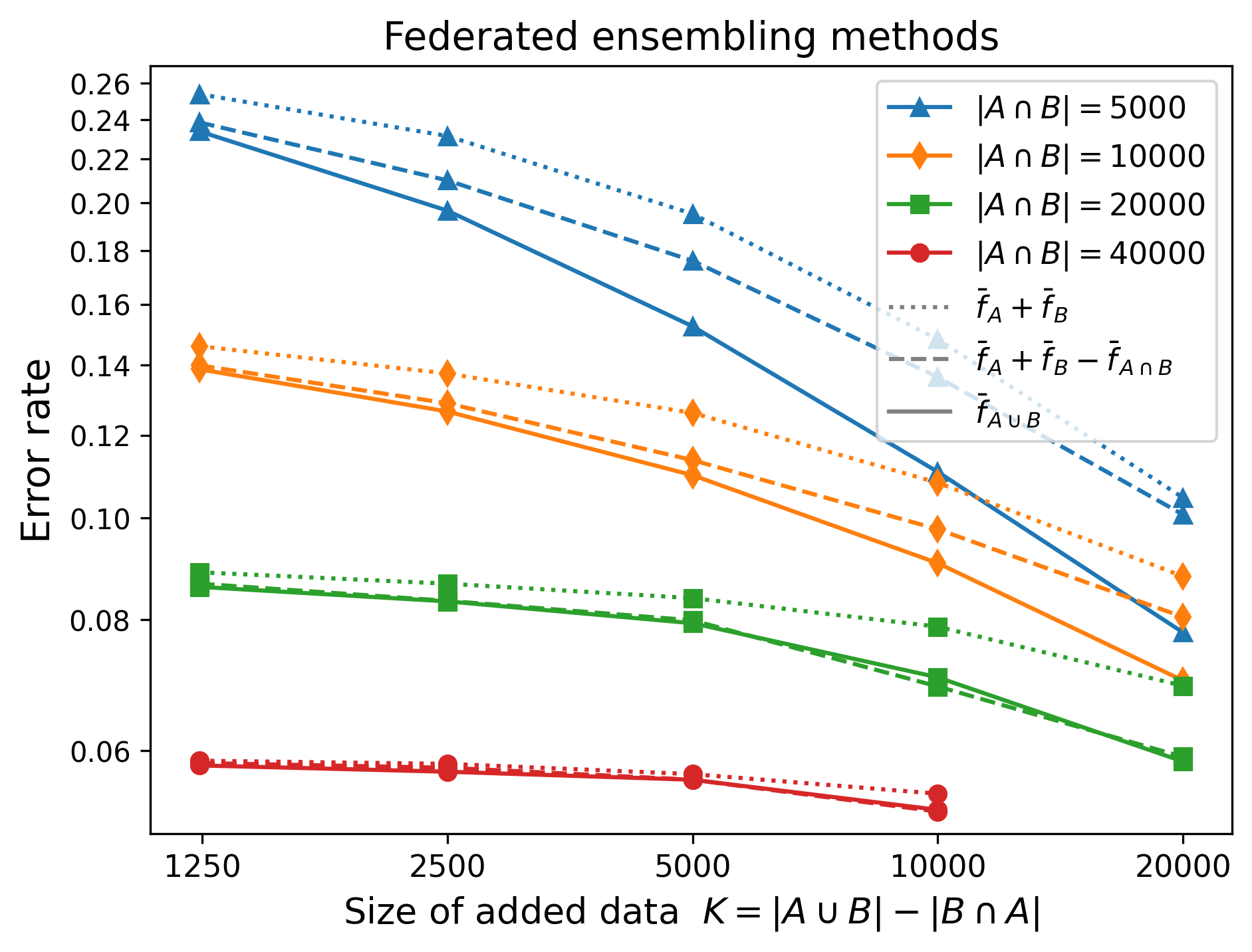
Figure 3. Federated learning formulas for ensemble learning across two nodes.
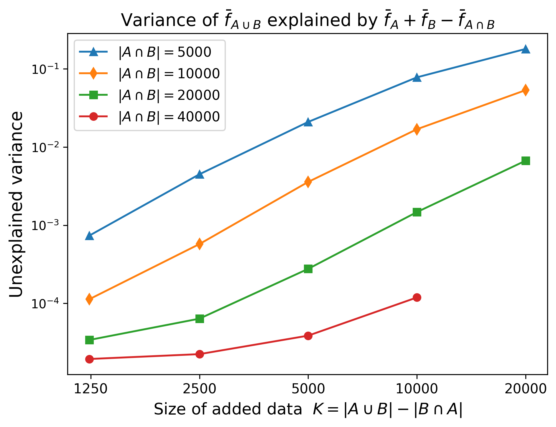
Figure 4. Unexplained variance. The relationship is super-linear. N = 8000 in every case.
In Figure 3 and 4 we display three values for each $(N, K)$ pair:
- The error rate given by naively ensembling $\bar f_A$ and $\bar f_B$.
- The error rate given by using Equation 1.
- The ideal-world error rate given by training on all of $A \cup B$.
We can make several observations:
- For $N \in {20000, 40000}$, it appears that Equation 1 is almost perfect, no matter the value of $K$.
- In general, the smaller $K/N$ is, the more accurate the formula is.
- The formula breaks down the most when $N$ is small and $K$ is large. For example, with $N, K = (5000, 10000)$ we have $\mathrm{acc}(\bar f_{A \cup B}) = 92.2\%$, but the formula gives only $\mathrm{acc}(\bar f_A + \bar f_B - \bar f_{A \cap B}) = 89.9\%$, which isn’t much better than the naive ensembling method which gives $\mathrm{acc}(\bar f_A + \bar f_B) = 89.5\%$.
(Note that the pair $(N = 40000$, $K = 10000)$ is missing, because this would require $|A \cup B| = 60,000$ which is impossible since the CIFAR-10 training set only contains 50,000 examples.)
Non-Random Subsets
In our experiments so far, the subsets $A$ and $B$ have been randomly sampled, which is in some sense an “easy case” for Equation 1. In this section, we test a few more pathological choices of subsets to see where the formula breaks down.
Scenarios
Recall that the CIFAR-10 training set contains 10 classes each with 5K examples, for a total of 50K examples.
We consider five scenarios. The first is just the “random 45K” scenario explored in the first section, and the remaining four are more pathological/non-random.
- (Baseline) Random 45K: Let $A$ be a random 45K examples. Let $B$ be a random 45K examples, such that the overlap with $A$ is 40K examples.
- Missing 500 cats and 500 dogs: Let $A$ be the full set, minus 500 random cats and 500 random dogs. Let $B$ be the full set, minus a different 500 random cats and 500 random dogs.
- Missing 2K cats and 2K dogs: Let $A$ be the full set, minus 2000 random cats and 2000 random dogs. Let $B$ be the full set, minus a different 2000 random cats and 2000 random dogs.
- Missing half of cats and dogs: Let $A$ be the 40K non-cat/dogs, plus 2500 cats and 2500 dogs. Let $B$ be the 40K non-cat/dogs, plus the other 2500 cats and 2500 dogs.
- Missing 4K cats or dogs: Let $A$ be the full set, minus 4000 random cats. Let $B$ be the full set, minus 4000 random dogs.
- Missing all cats or dogs: Let $A$ be the full set, minus all 5000 cats. Let $B$ be the full set, minus all 5000 dogs.
- Missing half of everything: Let $A$ be 25K random examples, and $B$ be the other 25K.
Results
| Scenario | $\bar f_{A \cap B}$ | $\bar f_A$ | $\bar f_B$ | $(\bar f_A + \bar f_B) / 2$ | $\bar f_A + \bar f_B - \bar f_{A \cap B}$ | $\bar f_{A \cup B}$ | Explained Var |
|---|---|---|---|---|---|---|---|
| 1 | 94.08% | 94.38% | 94.37% | 94.57% | 94.77% | 94.72% | 0.99990 |
| 2 | 94.50% | 94.69% | 94.63% | 94.65% | 94.76% | 94.72% | 0.99997 |
| 3 | 91.39% | 94.12% | 94.03% | 94.16% | 94.38% | 94.72% | 0.993 |
| 4 | 77.12% | 93.84% | 93.67% | 93.92% | 89.84% | 94.72% | 0.67 |
| 5 | 91.39% | 92.63% | 91.77% | 93.85% | 94.54% | 94.72% | 0.998 |
| 6 | 77.12% | 86.11% | 86.40% | 88.53% | 93.91% | 94.72% | 0.974 |
| 7 | n/a | 92.36% | 92.35% | 92.72% | 92.72% | 94.72% | 0.15 |
Note: In every scenario, $A \cup B$ is just the entire training set, hence why every scenario has $\mathrm{acc}(\bar f_{A \cup B}) = 0.9472$.
Also note: the $R^2$ for the deltas is:
- 0.993
- 0.992
Discussion
Equation 1 gives superior results to the naive ensembling in every scenario except for 4, where naive ensembling is significantly better.
The reason for this can be understood with some reasoning. In scenario 4, $A \cap B$ contains neither cats nor dogs, whereas both $A$ and $B$ contain many cats and dogs. Hence, $\bar f_{A \cap B}$ will always assign zero or slightly negative cat/dog logits, whereas the cat and dog logits assigned by $\bar f_A$ and $\bar f_B$ will have the usual scale. Therefore, $\bar f_A + \bar f_B - \bar f_{A \cap B}$ will have approximately double the scale for its cat and dog logits as compared to its other logits, leading to over-prediction of cats and dogs. Manual inspection confirms that this reasoning pans out, since $\bar f_A + \bar f_B - \bar f_{A \cap B}$ predicts either cat or dog 26% of the time, whereas the correct rate should be 20%.
This failure mode is the reason why we must add the qualification that data influence is locally additive. It is not additive if $A \cap B$ contains no examples of a subgroup which gets added in by both $A - (A \cap B)$ and $B - (A \cap B)$.
Case 2 has the same sized gap, but reversed so that $\bar f_A + \bar f_B - \bar f_{A \cap B}$ is dramatically better than $(\bar f_A + \bar f_B)/2$.
Conclusion
Overall, we have confirmed that the formula $\bar f_{A \cup B} = \bar f_A + \bar f_B - \bar f_{A \cap B}$ approximately holds when $A$ and $B$ are random subsets with a relatively large overlap. And we have shown that it breaks down in circumstances where $A$ and $B$ are not random, especially those where both $A$ and $B$ both introduce a new subgroup of data which is absent from their intersection.
Appendix
Additional Figures
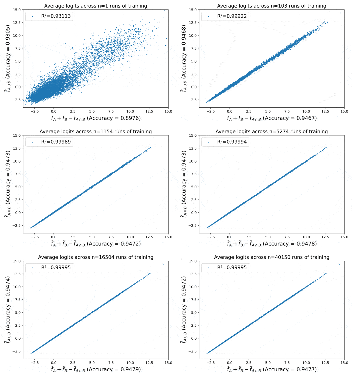
Here are some extra figures for the “random 45K” scenario which may be of interest to the reader.

Proofs
Lemma. Let $C$ and $D$ be disjoint sets of training data. Then assuming linear datamodeling, $\bar f_{C \sqcup D} = \bar f_C + \bar f_D$.
Proof. \begin{align} \bar f_{C \sqcup D}(x) &= \sum_{i=1}^n \theta_i \cdot 1\{(x_i, y_i) \in C \sqcup D\} \newline &= \sum_{i=1}^n \theta_i \cdot 1\{(x_i, y_i) \in C\} + \sum_{i=1}^n \theta_i \cdot 1\{(x_i, y_i) \in D\} \newline &= \bar f_C(x) + \bar f_D(x). \end{align}
Lemma. If $C \subset D$ then $\bar f_{D - C} = \bar f_D - \bar f_C$.
Proof. Similar.
Theorem. Assuming linear datamodeling, $\bar f_{A \cup B} = \bar f_A + \bar f_B - \bar f_{A \cup B}$ for all $A, B$, where we assume $\bar f_\varnothing = 0$.
Proof.
The set $A \cup B$ can be decomposed as the disjoint union $(A - (A \cap B)) \sqcup (B - (A \cap B)) \sqcup (A \cap B)$. Using the lemmas we therefore have \begin{align} \bar f_{A \cup B} &= \bar f_{(A - (A \cap B)) \sqcup (B - (A \cap B)) \sqcup (A \cap B)} \newline &= \bar f_{A - (A \cap B)} + \bar f_{B - (A \cap B)} + \bar f_{A \cap B} \newline &= \bar f_A + \bar f_B - \bar f_{A \cap B}. \end{align}