In this post I will contribute a result about neural network training which is surprising but probably not useful.
Introduction
Neural network training is an inherently random process (Summers & Dineen 2021). Every run of training, with the same hyperparameters, produces a unique network with unique behavior.
This variation makes it difficult to precisely study the effects of subtle changes in hyperparameters, like the learning rate.
For example, if we compare two runs of training with learning rates 0.5 and 0.55, then it is usually not possible to say what the effect of the different learning rates was, because any effects caused by such a small change will be drowned out by the inherent variability between runs.
This is in contrast to a field like structural engineering, where one can often say exactly what the effect will be of adding each additional increment of force to the structure.
As far as I’m aware, up to this point, it remains beyond the power of neural network science to say anything precise at all about the effect of changes in the learning rate.
It is even possible that the relationship between the learning rate and the outcome of training could be chaotic/fractal,
as @jaschasd suggests in his post on X. (the main figure of which is reproduced below)
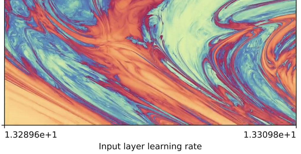
If we wish to succeed in our goal of turning the practice of deep learning into a mature engineering discipline, then it is of interest for us to begin by locating any precise true statement about the effect of the hyperparameters on practical neural network trainings.
In this post we contribute one such statement regarding the effect of the learning rate.
Experiment
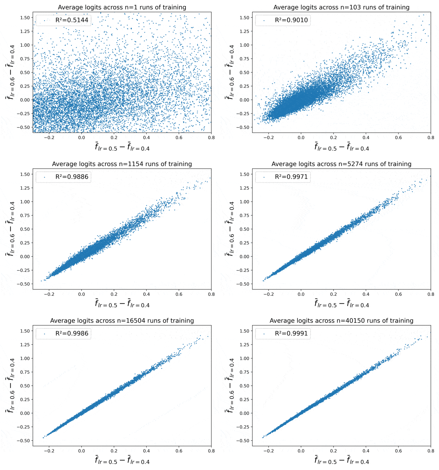
Figure 1. Learning rate has a locally linear effect on average neural network behavior across repeated runs of training.
This figure shows a certain empirical law of neural net behavior, as a function of the learning rate, which emerges when we take the average over repeated runs of training.
The experimental recipe which generated the figure is as follows.
- Train N networks on CIFAR-10 with learning rate 0.4, another N with lr=0.5, and another N with lr=0.6. All other hyperparameters besides the learning rate are kept fixed.
- This gives us 3 sets of N trained networks. Evaluate them all on the CIFAR-10 test-set, yielding three tensors of logit outputs, each of shape (N, 10000, 10) (because the test-set contains 10,000 examples).
- Take the average over the models dimension. This gives us three tensors of shape (10000, 10), which are the approximate mean logits for the three learning rates.
- Call these three tensors out4, out5, and out6. Then the X axis in the plot is (out5 - out4).flatten(), and the Y axis is (out6 - out4).flatten().
The following code may help provide further explanation.
# The last frame of the animation can be reproduced by the following.
def show_figure(outs_lr4, outs_lr5, outs_lr6):
    """
    Arguments:
    outs_lr4: the logits given by training with learning rate 0.4.
    outs_lr5: the same with lr=0.5.
    outs_lr6: the same with lr=0.6.

    We assume each of the three arguments is generated by executing
    40,000 repeated runs of training using the given learning rate,
    and then collecting all those trained networks' outputs on the
    CIFAR-10 test-set. Thus each argument is a tensor of shape
    (40000, 10000, 10).
    """
    assert outs_lr4.shape == (40000, 10000, 10)
    assert outs_lr5.shape == (40000, 10000, 10)
    assert outs_lr6.shape == (40000, 10000, 10)

    out4 = outs_lr4.mean(0)
    out5 = outs_lr5.mean(0)
    out6 = outs_lr6.mean(0)
    xx = (out5 - out4).flatten()
    yy = (out6 - out4).flatten()

    plt.scatter(xx.tolist(), yy.tolist(), s=1)
    plt.show()
To generate the animation I’m just increasing N = len(outs_lr4) (without the assert statements).
What we see in Figure 1 is that for large N, it becomes empirically true that (out6 - out4) $\approx 2\,\cdot\,\,$(out5 - out4)! The correlation between the two quantities reaches $R^2 = 0.9991$ for $N = 40000$.
Note that the underlying training configuration I am studying is (a slight modification of) my CIFAR-10 speed benchmark.
The Empirical Law
From this result we infer the following empirical law.
Let $\bar f_\eta$ be the mean neural network output across repeated runs of training using learning rate $\eta$. That is, for input $x$ we define $\bar f_\eta(x) := \mathbb E_{f \sim \mathcal A(\eta)}[f(x)]$ where $f \sim \mathcal A(\eta)$ denotes sampling a neural network trained using learning rate $\eta$, with fixed settings for all other hyperparameters.
Then we conjecture that the following relationship/law holds empirically:
$\bar f_{\eta + b} \approx \bar f_\eta + (b/a) \cdot (\bar f_{\eta + a} - \bar f_\eta)$
for small learning rate deltas $a$ and $b$.
If I had to come up with a summary for this law, it would be that “the learning rate has a locally linear influence on aggregate neural network behavior.”
Further Experiments
To validate this hypothesized law, I investigated a range of other learning rates from 0.1 to 1.5. I’ll omit the exact results and just report a summary:
I found that the law holds whenever $b/\eta$ and $a/\eta$ are relatively small. It begins to break down when you increase either much beyond $0.5$.
As you make $a/\eta$ and $b/\eta$ smaller, the correlation between the left- and right-hand sides of the law increases.
Discussion
Is this result surprising?
The first thing to observe is that if we take the limit as $a, b \to 0$, then what this law says is simply that the path traced out by the learning rate in function space is differentiable.
That is, that the path $\varphi(\eta) := \bar f_\eta$ admits first-order local approximations.
Is this surprising? I’m not sure. After seeing the result, it does seem obvious that it would be true. But before seeing it, I could just as easily have imagined that the picture would be more like a chaotic mess.
What’s more surprising is how smooth the path is. The learning rate 0.6 is of course 50% larger than 0.4. A priori, even if we feel that it is obvious that the path will be differentiable, it’s not obvious to me that it should be so smooth. In particular, Figure 1 showed that we get $R^2 = 0.9991$ between the two sides of the law with $\eta = 0.4$, $b = 0.2$, and $a = 0.1$.
So overall, I would say yes it is somewhat surprising.
Is this result useful?
Honestly I don’t think so. At least I’ve got no clue how to make it useful.
Perhaps it will be useful in the form of enabling useful future discoveries which are further down the scientific tree.
I would definitely not look forward to trying to sell the average reviewer on the value of this result. I don’t think I could do it without the help of an experienced coauthor.
Appendix
Added 05/14/24.
In this section we will consider a few more questions.
Question 1
Could this relationship have a trivial explanation, like, perhaps the deltas in Figure 1 are just a simple function of the original logit?
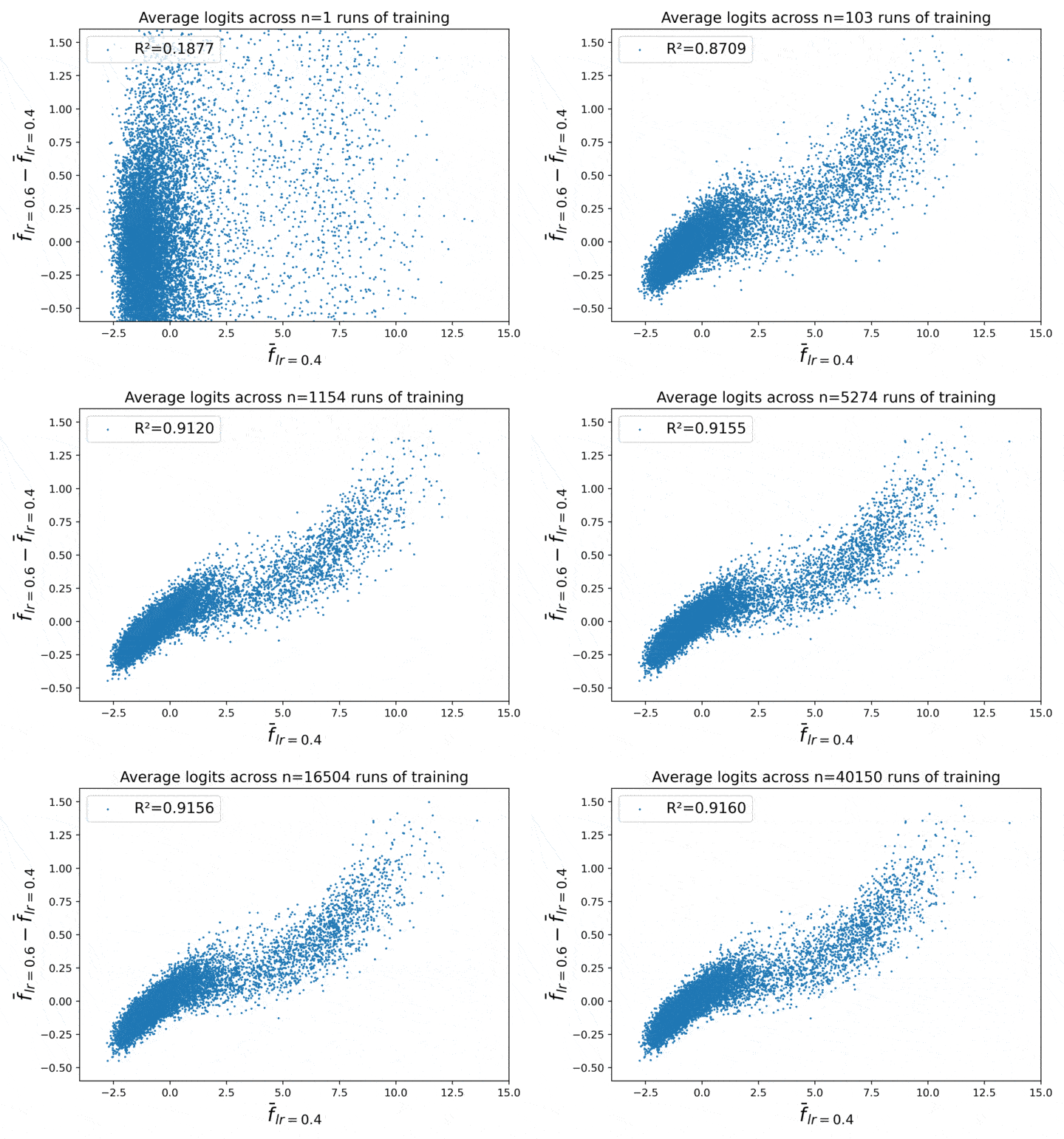
Figure 2. The delta vs. original logit scale. There is no strong relationship.
Nope, not as far as I can tell.
Question 2
The main section indicates that the following limit is well-defined:
\begin{equation} \Delta(x, \eta) := \lim_{a \to 0} \frac{\bar f_{\eta + a}(x) - \bar f_\eta(x)}{a} \end{equation}
And is smooth enough so that $\bar f_{lr=0.6}(x) \approx \bar f_{lr=0.4}(x) + 0.2 \cdot \Delta(x, 0.4)$.
What is the meaning of this object? Is there anything we can say about which image features cause it to be larger, or smaller?
In other words: What kind of features does the network become more sensitive to as we increase the learning rate?
Our experimental recipe will be as follows:
- We will collect a set of 1000 dogs in the CIFAR-10 training set which have middling mean confidence, in particular, dogs $x$ such that $\bar f_{lr=0.4}(x)[5]$ is between its 40th and 60th percentile.
- We will visualize the top and bottom 24 such dogs, as ordered by their dog-logit delta $\bar f_{lr=0.6}(x)[5] - \bar f_{lr=0.4}(x)[5]$.
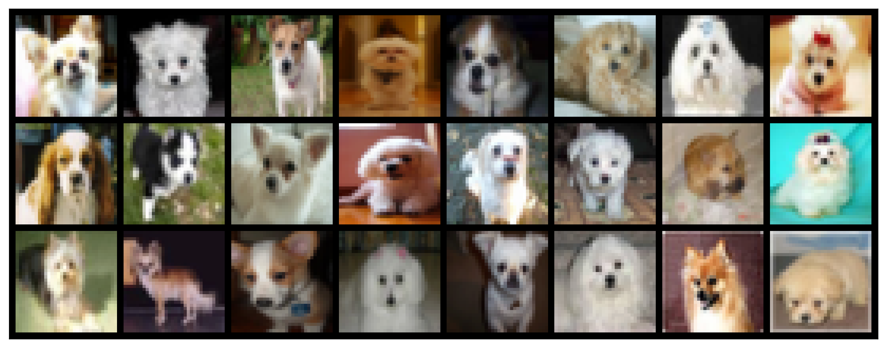 Figure 3. The dogs whose dog logit was most increased by increasing $\eta$ from $0.4$ to $0.6$.
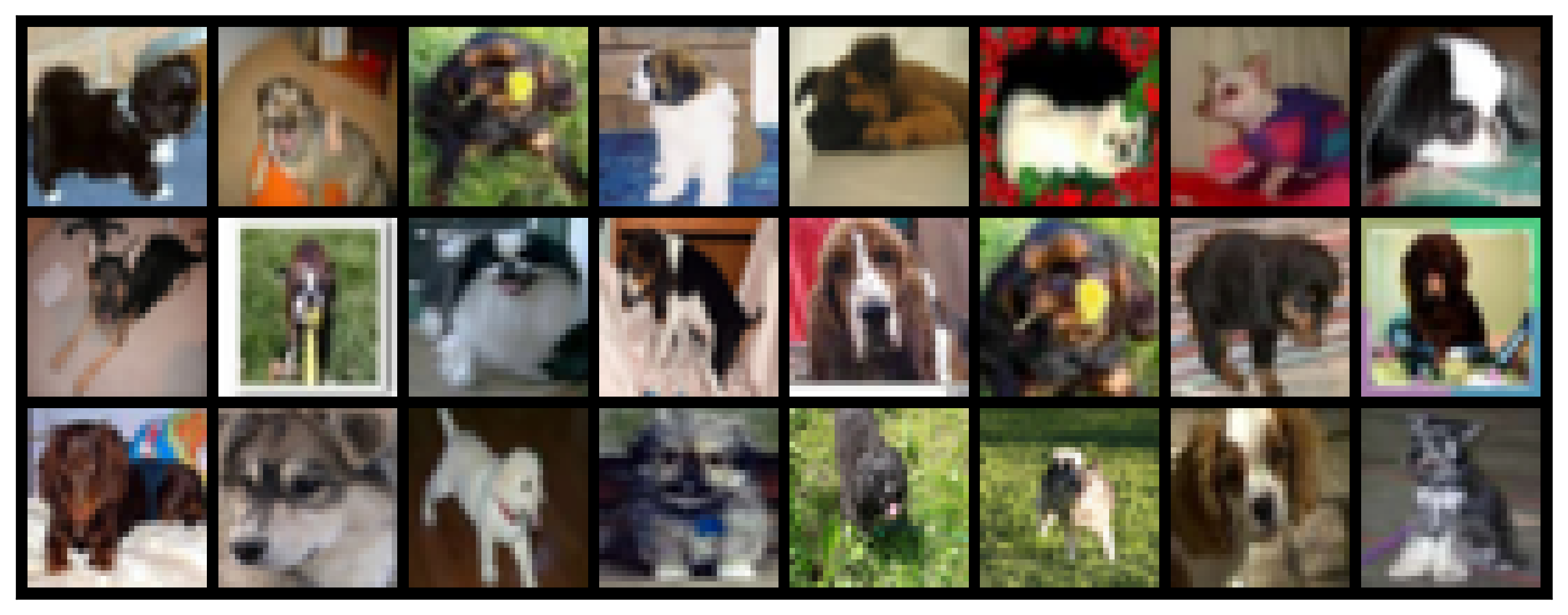 Figure 4. The dogs whose dog logit was least increased by increasing $\eta$ from $0.4$ to $0.6$.
- On average, the top 24 images have their dog-logit increase by 0.8 when increasing $\eta$ from 0.4 to 0.6. The bottom 24 increase by only 0.2.
- With $\eta = 0.4$, the second 24 dogs are all more confident than the first.
- With $\eta = 0.6$, the first 24 dogs are all more confident than the second.
There does seem to be a pattern here. Repeating for automobile gives the following:
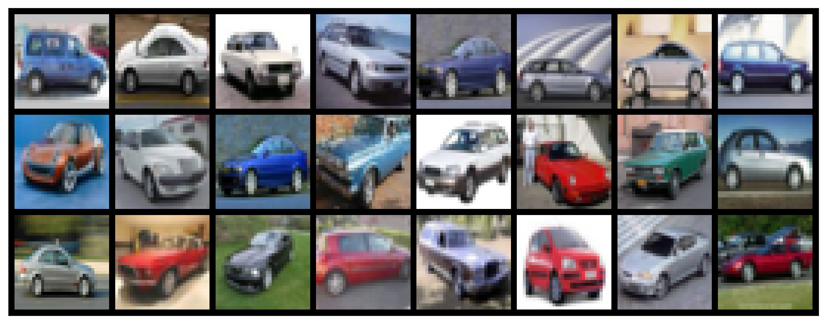 Figure 5. The automobiles whose automobile logit was most increased by increasing $\eta$ from $0.4$ to $0.6$.
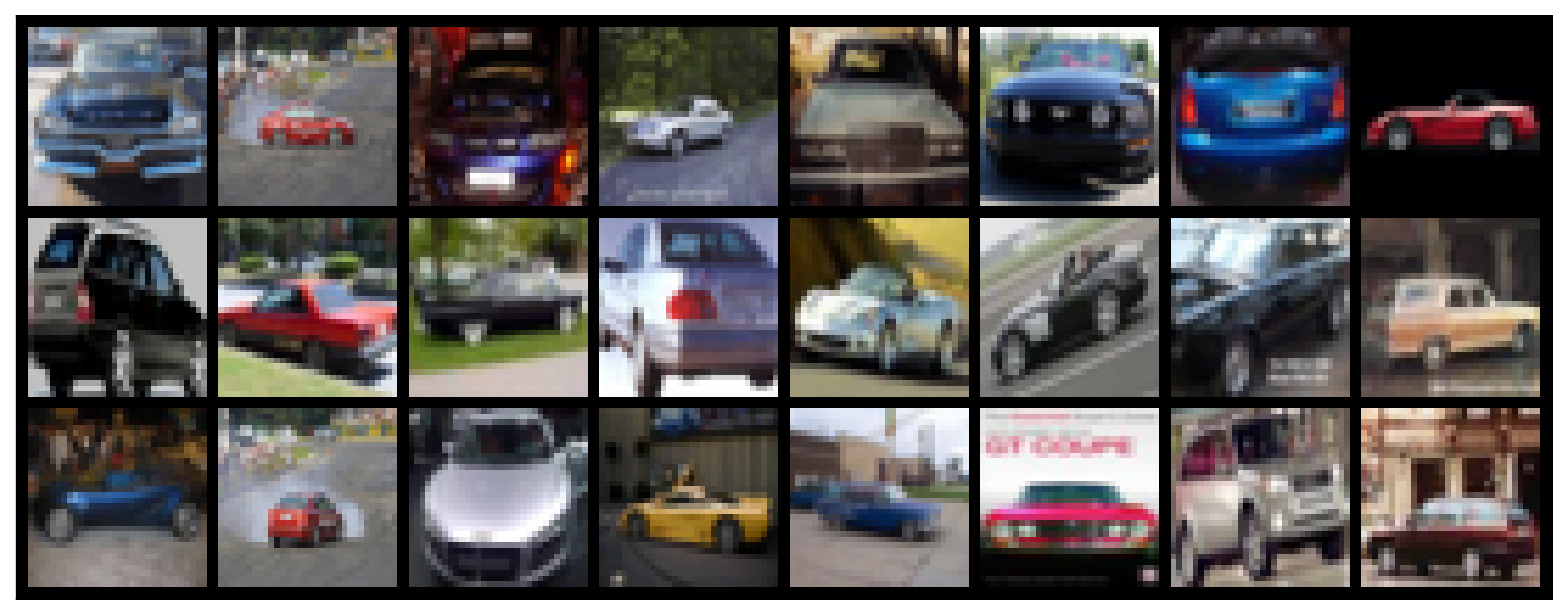 Figure 6. The automobiles whose automobile logit was least increased by increasing $\eta$ from $0.4$ to $0.6$.
- On average, the top 24 images have their automobile-logit increase by 0.9 when increasing $\eta$ from 0.4 to 0.6. The bottom 24 increase by only 0.2.
- Again, the top 24 images are all more confident for $\eta = 0.6$, and the bottom 24 more confident for $\eta = 0.4$.
What is the pattern here?
When thinking about this question, I find it important to remember that in each case, the top and bottom images are both assigned a similar middling level of confidence.
It’s not just that the top images are more “normal” or “easier”. The network sees them as being of similar difficulty.
I also find it important to remember that both $\eta = 0.4$ and $\eta = 0.6$ lead to nearly the exact same accuracy. So what’s different here is really just the network’s sensitivity to one kind of feature over another, rather than the overall performance of the network.
Rather, what seems salient to me about the top 24 images is that they are taken from a “typical angle/distance”. In the top 24 images, what I notice is that all the objects occupy a similar portion of the frame.
I’m tempted to say that higher learning rate leads to better performance on “typical” examples and worse performance on “atypical” examples.
Why is this the case? I’m not sure.